Multiprocessor Classification: Flynn Taxonomy, Memory Models and Exam-Style Worked Examples

Multiprocessor classification is not one four-item list: instruction streams, memory organisation, access-time uniformity, and coupling are independent axes. Multiprocessors in COA: Concepts, Amdahl's Law and Cache Coherence Worked Examples connects interconnects, Amdahl speedup, and cache coherence. Classification questions begin by identifying which axis the evidence belongs to; mixing the axes produces plausible but wrong labels. A four-lane SIMD trace and a four-node NUMA calculation make that evidence test concrete; use the GATE CS Exam route to place the topic within broader preparation.

Multiprocessor classification: choose the axis before the label

A processing element is a processor, core, or execution lane capable of doing work in the model stated by the question. Parallel execution means that work overlaps in time. Physical processor count alone does not settle the classification. The same four units could apply one shared operation to four data items or execute four independent operations.

Use three separate axes:

• Instruction and data streams: Flynn's SISD, SIMD, MISD, and MIMD.

• Memory visibility and access time: shared or distributed memory, then UMA or NUMA where a shared address space is involved.

• Communication and coupling: tightly coupled or loosely coupled.

These labels answer different questions. One more separation worth keeping: an addressing mode tells a single instruction how to locate its operand, so it says nothing about how multiple processors coordinate.

Flynn's taxonomy: SISD, SIMD, MISD and MIMD

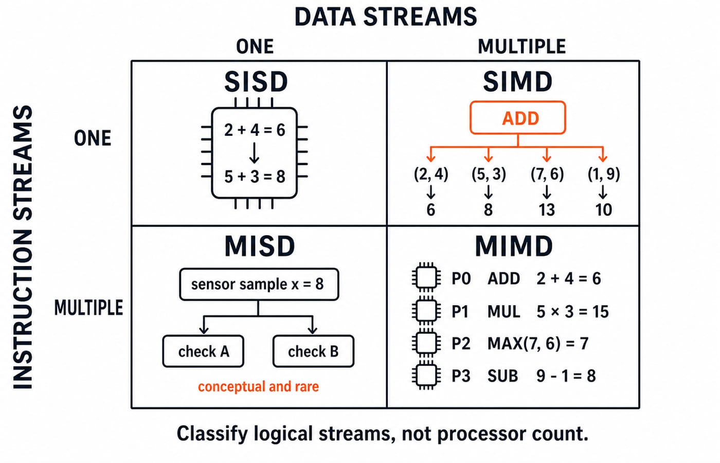
Flynn's taxonomy is a two-by-two classification of logical instruction and data streams.

SISD can be one core calculating 2 + 4 = 6, then later 5 + 3 = 8. SIMD can be four lanes receiving the same ADD for four element pairs. In a conceptual MISD example, two different checks process the same sensor sample stream; clear textbook MISD systems are rare. MIMD can have separate cores concurrently performing ADD, multiplication, maximum, and subtraction on different inputs.

The decision test is simple: count logical instruction streams first, then data streams. A brand name, core count, or the word “parallel” is not enough.

SIMD worked example: add two four-element vectors

Let A = [2, 5, 7, 1], B = [4, 3, 6, 9], with processing elements PE0 to PE3. In one abstract execution step, one ADD instruction is issued to all four elements. Lane PEi reads A[i] and B[i], then writes C[i]. Memory-transfer time, divergence, and communication are outside this teaching model.

Each lane performs its assigned addition:

• PE0: 2 + 4 = 6

• PE1: 5 + 3 = 8

• PE2: 7 + 6 = 13

• PE3: 1 + 9 = 10

Therefore, C = A + B = [6, 8, 13, 10]. All four results form the same output vector. This trace is SIMD because it has one logical instruction stream and four data-element pairs, not merely because four processing elements exist.

Now hold the processor count at four but change the instruction streams. Let P0 perform ADD, 2 + 4 = 6; P1 perform MUL, 5 x 3 = 15; P2 perform MAX, MAX(7,6) = 7; and P3 perform SUB, 9 - 1 = 8. Independent operations on separate inputs make this trace MIMD. The processor count stayed fixed while the instruction streams changed.

Shared memory, distributed memory, UMA and NUMA

In a shared-memory organisation, processors communicate through a common address space. In a distributed-memory organisation, nodes keep private memories and exchange explicit messages. Distributed memory is not a Flynn cell, and shared memory does not guarantee uniform access time.

Within shared memory, UMA means that the stated main-memory access time is independent of both the requesting processor and the target memory location, under the comparison's fixed assumptions. NUMA means that access time depends on where the memory is located relative to the requester. Private caches and contention can affect observations in real machines, but the numerical model below holds them constant. The Cache Memory: Mapping and Hit Ratio note develops the cache side separately.

A shared-memory multiprocessor is conventionally tightly coupled because its processors coordinate through a common address space and close interconnect. Private-memory nodes using messages are loosely coupled. Treat this as an architectural tendency because hybrid systems need not fit one pure box.

UMA versus NUMA worked example: calculate average access time

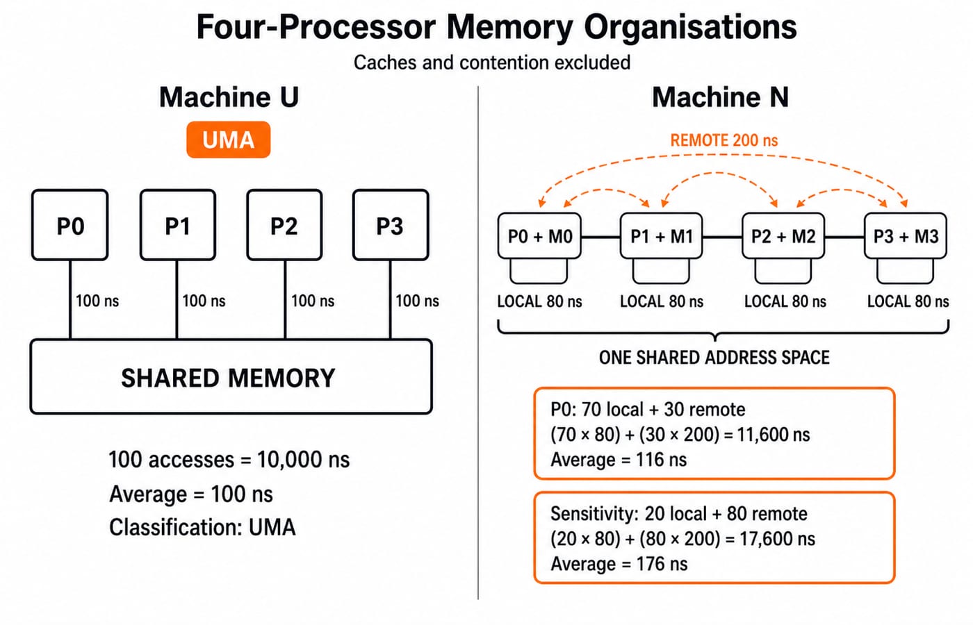
Machine U has four processors and one shared address space. With caches and contention excluded, every processor reaches every main-memory block in 100 ns. It is UMA. For 100 accesses:

100 x 100 ns = 10,000 ns

Average access time is 10,000 / 100 = 100 ns.

Machine N has four nodes in one shared address space. Local memory takes 80 ns, while another node's memory takes 200 ns. It is NUMA because latency changes with location. For P0's 100 references, with 70 local and 30 remote:

(70 x 80) + (30 x 200) = 5,600 + 6,000 = 11,600 ns

Average access time is 11,600 / 100 = 116 ns.

As a sensitivity check, suppose only 20 references are local and 80 are remote:

(20 x 80) + (80 x 200) = 1,600 + 16,000 = 17,600 ns

The average is 17,600 / 100 = 176 ns. Locality changes the observed NUMA average. The NUMA label alone does not promise a fixed speed advantage.

Multiprocessor classification traps: repair the shortcut

“Same program” does not prove SIMD when cores have independent control. A shared data set is not one stream when processors handle partitions independently. Classify the trace in front of you. Anchors: one ADD across four pairs is SIMD, different operations on different inputs are MIMD, and 80 ns local versus 200 ns remote means NUMA.

How exams test multiprocessor classification

Prompts may ask for the Flynn matrix, trace classification, a vector-to-SIMD match, a coupling distinction, a memory model inferred from latency, or rejection of mixed axes.

For this recognition drill, give the evidence with the label:

1. One ADD across (2,4), (5,3), (7,6), (1,9) is SIMD.

2. ADD, MUL, MAX, and SUB on separate inputs is MIMD.

3. All main-memory paths at 100 ns describe UMA.

4. 80 ns local and 200 ns remote describe NUMA.

The related Pipelining in Computer Architecture Explained note separates stage overlap from Flynn's logical streams. Use timed questions to practise giving the evidence with each label.

Multiprocessor classification: the short version and next step

Retrieve the axes in this order: streams -> memory -> access time -> coupling. The four-lane ADD produces [6, 8, 13, 10] and is SIMD. The NUMA workload with 70 local and 30 remote references averages 116 ns.

For a structured route through wider Computer Organisation, use GATE Guidance by Sanchit Sir. Then continue with Pipelining in Computer Architecture Explained and keep its stage overlap separate from Flynn's stream classification.