Pipelining in Computer Architecture: the 5-stage pipeline, speedup, and hazards
Pipelining in computer architecture: the 5-stage pipeline, speedup and throughput formulas, CPI, structural, data and control hazards, and forwarding.
KnowledgeGate Team
Exam prep & CS education
Updated 25 Jul 20265 min read60 views
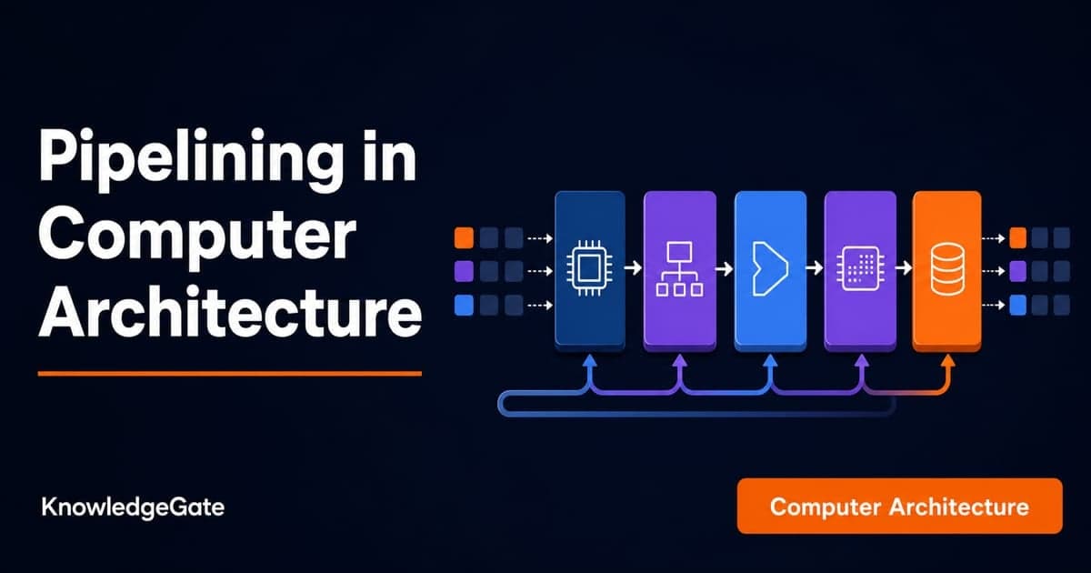
Pipelining is one of the highest-yield topics in Computer Organisation and Architecture for GATE, and it is almost pure arithmetic once you understand the model. The aspirants who lose marks here do so by memorising the speedup formula without knowing where the "minus one" comes from, or by ignoring the stalls that hazards inject. The whole model is small: five stages, one expression for total time, (k + n − 1) cycles for n instructions, and a short list of hazards that add cycles back on.
Pipelining: the classic 5-stage pipeline
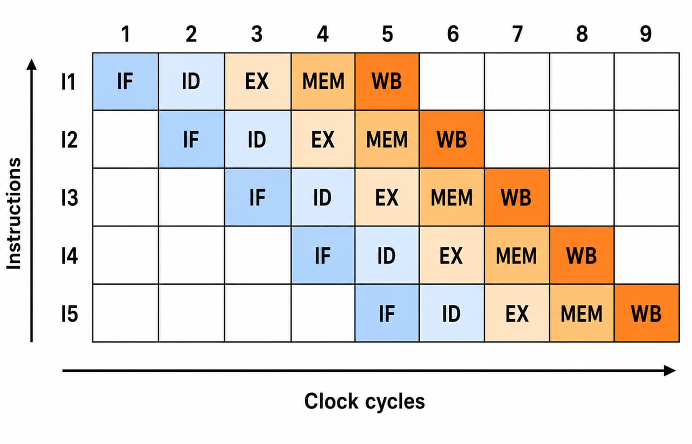
Pipelining overlaps the execution of consecutive instructions the way an assembly line overlaps cars. A single instruction still passes through every stage; what changes is that while instruction 1 is in stage 2, instruction 2 can already be in stage 1. The classic RISC pipeline has five stages:
IF (instruction fetch): read the instruction from memory.
ID (instruction decode): decode it and read the register operands.
EX (execute): perform the ALU operation or compute an address.
MEM (memory access): read or write data memory.
WB (write back): write the result into a register.
Each stage is separated by a pipeline register that latches the intermediate result, so all five stages run in the same clock cycle on five different instructions. That one structural idea is what every pipelining numerical rests on, and the Computer Architecture learn module sets it beside the control-unit and memory-hierarchy topics that reuse the same timing model.
Pipelining speedup, throughput and CPI
Consider k pipeline stages, each taking one clock cycle of period τ, executing n instructions.
A non-pipelined processor takes k cycles per instruction, so total time is n × k × τ.
A pipelined processor fills the pipe in k cycles for the first instruction, then completes one instruction every cycle thereafter, so total time is (k + n − 1) × τ. That "minus one" is because the first instruction already accounts for one of the n completions.
Speedup is the ratio:
Speedup = (n × k) / (k + n − 1)
As n grows large, the fraction approaches k, the number of stages. That is the ideal speedup, and no pipeline reaches it exactly because of the fill-and-drain overhead and hazards.
Throughput is instructions completed per unit time. Over the whole run it is n / ((k + n − 1) × τ), and in steady state that approaches 1 / τ, one instruction per clock cycle. CPI (cycles per instruction) is 1 in an ideal pipeline; every stall pushes it above 1, which drags steady-state throughput down to 1 / (CPI × τ). Computing the effective CPI is the heart of most exam numericals.
Pipeline hazards: structural, data and control
A hazard is any condition that stops the next instruction from executing in its intended cycle. There are three kinds.
Structural hazard: two instructions need the same hardware in the same cycle, for example a single memory port serving both an instruction fetch and a data access. Separate instruction and data caches remove this one.
Data hazard: an instruction needs a result that an earlier, still-in-flight instruction has not yet written back. The common case is read-after-write (RAW): instruction 2 reads a register that instruction 1 is about to write.
Control hazard: a branch changes the instruction flow, but the pipeline has already fetched the instructions after the branch before knowing whether the branch is taken.
Forwarding, stalls and bubbles
The naive fix for a data hazard is to stall: hold the dependent instruction until the result is written back, inserting empty cycles called bubbles. Bubbles waste throughput, so real pipelines add forwarding (also called bypassing): the ALU result is routed directly from the EX or MEM stage output back to a later instruction's input, without waiting for write-back. Forwarding removes most RAW stalls. The one it cannot fully hide is a load followed immediately by a use of the loaded value, which still costs one bubble, because the data is not available until after MEM.
Branch handling attacks control hazards. Options range from stalling until the branch resolves, to branch prediction (guess taken or not-taken and squash the wrong-path instructions if wrong), to a delayed branch that always executes the instruction after the branch. Each trades hardware for fewer wasted cycles.
Pipelining speedup: a worked example
Take a 5-stage pipeline, n = 1000 instructions, and a clock period τ = 2 ns.
Non-pipelined time = n × k × τ = 1000 × 5 × 2 = 10,000 ns.
Pipelined time = (k + n − 1) × τ = (5 + 1000 − 1) × 2 = 1004 × 2 = 2008 ns.
Speedup = 10,000 / 2008 ≈ 4.98, close to the ideal 5 because n is large.
Throughput = n / pipelined time = 1000 / 2008 ≈ 0.498 instructions per ns, just under the ideal 1 / τ = 0.5.
Now add hazards. Suppose 20 percent of instructions incur a one-cycle stall. The effective CPI becomes 1 + 0.20 × 1 = 1.2 cycles per instruction. The pipelined execution time in steady state is then approximately n × CPI × τ = 1000 × 1.2 × 2 = 2400 ns, the realistic speedup drops to 10,000 / 2400 ≈ 4.17, and throughput falls with it to 1 / (1.2 × 2) ≈ 0.417 instructions per ns. This gap between ideal and effective speedup is exactly what examiners want you to compute.
How pipelining is tested in GATE, NET and placements
GATE CS almost always includes a pipelining numerical: given the stage delays, find the clock period (the slowest stage plus latch delay sets it), then compute speedup, throughput, or total cycles for a given instruction mix with a stated stall frequency. Reading a space-time diagram to count stall cycles is a recurring question type, and the diagram above is the exact shape you will be handed.
UGC NET Computer Science keeps it conceptual: name the three hazard types, explain forwarding, and match a scenario to its hazard. Placement tests ask the same conceptually and sometimes tie pipelining to the memory system, since a pipeline stalls waiting on the cache memory mapping and hit ratio and on the broader memory hierarchy behind it.
The short version
Understand the model and the arithmetic follows: a k-stage pipeline runs n instructions in (k + n − 1) cycles, giving a speedup that approaches k, minus whatever hazards steal. Learn the three hazard types, know that forwarding hides most data hazards but not a load-use, and practise computing effective CPI from a stall frequency. Work several numericals by hand, because that is exactly what the exam gives you. For a GATE-depth COA sequence with solved pipelining problems, GATE Guidance by Sanchit Sir is built for it, and the GATE CS exam category covers the rest of the paper.
Keep learning

Data Manipulation Micro-Operations in COA: Arithmetic, Logic and Shift Operations Worked Step by Step
Learn a fixed-width method for tracing arithmetic, logic, and shift micro-operations. Every example tracks register values, result bits, carry, and overflow.
Updated 19 Oct 20265 min readComputer Organization & Architecture
Assembly Language and Assembler Design: Two-Pass Translation with a Complete Worked Example
Follow a 16-bit Basic Computer program through pass one, pass two, hexadecimal encoding and execution, with every symbol, address and result shown.
Updated 15 Oct 20266 min readComputer Organization & Architecture
Computer Classification and Flynn’s Taxonomy: The Four Classes with a Worked Vector Example
A machine can belong to several computer classes at once. Learn the four classification axes, Flynn’s matrix, vector and multicore traces, and exam traps.
Updated 11 Oct 20266 min readComputer Organization & Architecture
Programmed I/O: Polling, CPU Utilisation, Worked Examples and GATE Question Patterns
Follow one programmed-input transfer from control write to data read, then calculate how many polls one word costs and what a longer poll period buys.
Updated 7 Oct 20266 min readComputer Organization & Architecture