Artificial Neural Networks: Complete Guide with Worked Examples for GATE and Interviews
Turn ANN diagrams into numbers. Work through a neuron, activation derivatives, OR and XOR, one gradient update, backpropagation and parameter counts.
KnowledgeGate Team
Exam prep & CS education
Updated 2 Aug 20267 min read
You may sketch a neural network from memory, yet stall when asked for its output, one weight update, or its trainable parameter count. Exams and interviews test artificial neural networks through arithmetic and short derivations. The fix is arithmetic you have done yourself: one neuron's output of 0.668, its activation derivative, a single weight update, and the 26 trainable parameters of a 3-4-2 network.
1. The artificial neuron: one weighted sum, one activation
An artificial neuron first computes a weighted sum, then applies an activation function:
z = w1x1 + w2x2 + ... + wnxn + b, followed by a = f(z).
In the biological analogy, inputs act like dendrites, weights like synapse strengths, and the activation like a firing decision.
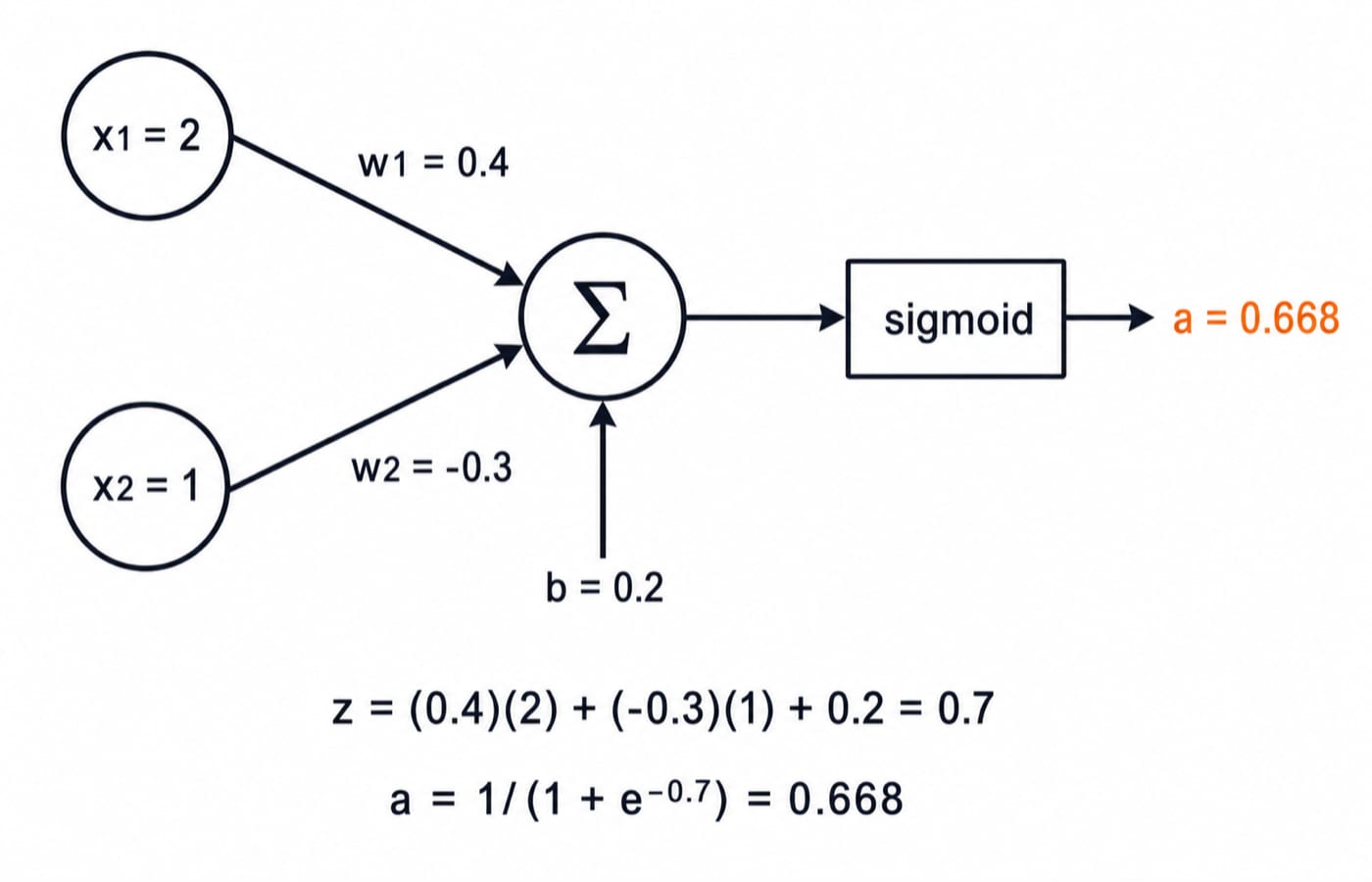
Take x1 = 2, x2 = 1, w1 = 0.4, w2 = -0.3, and b = 0.2:
z = (0.4)(2) + (-0.3)(1) + 0.2 = 0.8 - 0.3 + 0.2 = 0.7
With sigmoid activation:
a = 1/(1 + e^-0.7) = 0.668
Weights and biases are the learnable quantities. Training means adjusting them to reduce a loss.
2. Activation functions: the four that get asked
Four activation functions cover the foundations:
Function | Output and derivative | What to remember |
|---|---|---|
Step | 0 or 1, not differentiable at the threshold | Classic perceptron, unsuitable for ordinary gradient learning |
Sigmoid | Range 0 to 1, derivative | Smooth, but saturates when |
tanh | Range -1 to 1, derivative 1 - a^2 | Zero-centred, but still saturates |
ReLU |
| Cheap, but a neuron can get stuck at zero |
For our neuron, a = 0.668. Its sigmoid derivative is:
a(1 - a) = 0.668 x 0.332 = 0.222
Keep that value for the weight update. Also remember the interview answer: stacking purely linear layers still produces one linear map. Non-linearity is what gives depth its power.
3. Perceptron learning and linear separability: OR works, XOR breaks
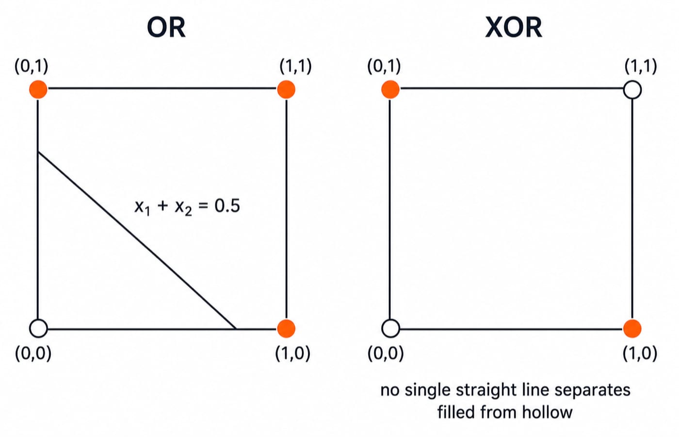
Use a step activation that outputs 1 when z >= 0. An OR perceptron can take w1 = 1, w2 = 1, and b = -0.5.
x1 | x2 | z = x1 + x2 - 0.5 | Output |
|---|---|---|---|
0 | 0 | -0.5 | 0 |
1 | 0 | 0.5 | 1 |
0 | 1 | 0.5 | 1 |
1 | 1 | 1.5 | 1 |
The decision boundary is x1 + x2 = 0.5. One perceptron draws one straight boundary, which is the meaning of linear separability.
Perceptron learning finds such weights on its own. The rule is wi(new) = wi + eta(t - y)xi, fired only on an example the perceptron gets wrong, with the bias updated as a weight on a constant input of 1. Start from w1 = 0.2, w2 = 0.2, b = -0.5 and eta = 0.4. On input (1,0) with target 1, z = 0.2 - 0.5 = -0.3, so the output is 0 and the error t - y = 1:
w1(new) = 0.2 + 0.4 x 1 x 1 = 0.6w2(new) = 0.2 + 0.4 x 1 x 0 = 0.2b(new) = -0.5 + 0.4 x 1 = -0.1
One update settles it. Those weights give z values of -0.1, 0.5, 0.1 and 0.7 across the four rows, which is exactly OR. Its boundary 0.6x1 + 0.2x2 = 0.1 is not the line above, and need not be, since many straight lines separate OR.
XOR puts (0,0) and (1,1) in one class, with (0,1) and (1,0) in the other. No straight line separates those classes, so one perceptron cannot compute XOR. One hidden layer of two suitable neurons can. Minsky and Papert's 1969 book Perceptrons set out these limits, and it helped cool neural-network research for a time.
4. One full gradient-descent weight update, every number shown
Reuse the first neuron with target t = 1, squared-error loss E = (1/2)(t - a)^2, and learning rate eta = 0.5.
Forward pass:
z = 0.7,a = 0.668, andt - a = 0.332.Loss:
E = 0.5 x 0.332^2 = 0.055.Local delta:
delta = (t - a) x a(1 - a) = 0.332 x 0.222 = 0.074.Update rule:
wi(new) = wi + eta x delta x xi.
Keeping full precision during the calculation and rounding only the displayed answers:
w1(new) = 0.4 + 0.5 x 0.074 x 2 = 0.474w2(new) = -0.3 + 0.5 x 0.074 x 1 = -0.263b(new) = 0.2 + 0.5 x 0.074 = 0.237
With the unrounded updated values, the new forward pass is:
z(new) = (0.473567)(2) + (-0.263216)(1) + 0.236784 = 0.921
a(new) = sigmoid(0.921) = 0.715
The output has moved from 0.668 towards target 1, and the loss has fallen from 0.055 to about 0.041. This single-neuron update is the innermost operation of backpropagation. A deep network applies it through the chain rule.
5. Multi-layer networks, backpropagation, and parameter counting
The input layer holds values and does no neuron computation. Hidden layers transform representations, and the output layer produces the prediction. Fully connected means every neuron feeds every neuron in the next layer. Commonly, depth counts computing layers, not the input layer.
Backpropagation has three moves: run a forward pass, compute output-layer deltas, then pass the error signal backwards. A hidden neuron's delta equals the sum of downstream deltas weighted by its outgoing connections, multiplied by its own activation derivative.
Put a number on that. Take the output delta of 0.074 computed above, an outgoing weight of 0.8 from hidden neuron h to that output neuron, and h's own sigmoid output of 0.6. Then delta_h = 0.074 x 0.8 x 0.6(1 - 0.6) = 0.074 x 0.8 x 0.24 = 0.0142, and every weight feeding h uses the same update rule with delta_h in place of delta.
Now count parameters in a 3-4-2 network:
Weights:
3 x 4 + 4 x 2 = 12 + 8 = 20Biases:
4 + 2 = 6Total trainable parameters:
20 + 6 = 26
For consecutive layer sizes, add n_in x n_out + n_out for every layer pair.
One epoch processes the full training set; an iteration performs one update. Stochastic gradient descent uses one example, batch gradient descent uses the full set, and mini-batch training sits between them. Overfitting means training improves while unseen-data performance worsens, so we retain a validation split.
6. Traps that cost marks
Layer count ambiguity: A
3-4-2network is a two-layer network under the computing-layer convention. If wording is unclear, state your convention.Missing biases: The example has 26 parameters, not 20.
Wrong sigmoid input: The derivative is
a(1 - a), using activationa = 0.668, not pre-activationz = 0.7.Inverted perceptron claim: A perceptron can learn linearly separable OR and AND, but not XOR.
Learning-rate confusion:
etais chosen as a hyperparameter. Too large can oscillate or diverge; too small learns slowly.Update-sign slip: If
delta = (t - a)f'(z), use the plus update shown above. If you define the error term as(a - t)f'(z), use gradient subtraction. Derive the sign rather than mixing conventions.
7. How GATE, NET, and interviews test ANNs
GATE's official papers and syllabus portal lists multi-layer perceptrons and feed-forward neural networks under Machine Learning in the DA paper, Data Science and Artificial Intelligence. The CSE core paper carries no ANN section. So CSE students should treat ANNs as preparation for a DA-paper switch, for UGC NET and CS teaching-recruitment syllabi, and for machine-learning interviews. Paper lists change between cycles, so confirm yours on the official portal.
Numerical questions can ask for a forward output, one gradient update, or a parameter count. Concept questions test separability, activation properties, and why XOR needs a hidden layer. For a solved set in exam wording, work through Artificial Neural Networks MCQs: 10 Solved Questions. UGC NET aspirants can also see where ANNs rank against the rest of Paper 2 in UGC NET Computer Science High-Yield Topics.
For interviews, prepare crisp explanations of why non-linearity matters, sigmoid versus ReLU, XOR, and backpropagation as weighted blame passed backwards.
8. The short version and your next step
A neuron is a weighted sum plus an activation. Non-linearity is essential. One perceptron draws one straight boundary. Learning repeats one delta-and-update step. Parameter counting means adding weights and biases for each adjacent layer pair.
If you are deciding how ANN preparation fits your GATE paper plan, continue with GATE Guidance by Sanchit Sir. If your goal is machine-learning and generative-AI interview preparation, use AI & ML for Placements | Generative AI Placement Course. For the wider syllabus around it, browse GATE CS Exam Preparation.
Keep learning
Problem Representation in AI: State Space, Worked Water-Jug Example and Exam Traps
Learn how states, operators, goals and costs turn a verbal task into a search problem. The worked water-jug trace separates valid states from reachable ones.
Updated 23 Oct 20265 min readML & Data Science
Foundations and Evolution of AI: Approaches, Timeline and a Worked Rational-Agent Example
Build a connected map of AI foundations, historical shifts and major paradigms, then calculate how a rational agent chooses under uncertainty.
Updated 19 Oct 20266 min readML & Data Science

Natural Language Processing Explained: Pipeline, TF-IDF Worked Example and Exam Patterns
Start from raw text, build BoW and TF-IDF vectors, compute cosine similarity, examine ambiguity, and finish with evaluation and exam-style checks.
Updated 15 Oct 20266 min readML & Data Science

Fundamentals of Planning in AI: STRIPS, State-Space Search and a Worked Blocks World Plan
Build a planning problem from facts, actions and goals, then follow every add and delete effect through a complete six-step Blocks World solution.
Updated 11 Oct 20266 min readML & Data Science