Pandas Basics in Python: Build, Clean and Analyse a DataFrame Step by Step
Follow one student dataset from its first DataFrame to a clean city summary, while learning how selection, missing values and vectorised calculations really work.
KnowledgeGate Team
Exam prep & CS education
Updated 24 Sep 20265 min read

Filtering, missing-value repair and city-wise aggregation are easier to understand when each operation acts on the same table. The working DataFrame contains five students, four source columns and one missing score. Cleaning fills that score with 85.0; a vectorised calculation adds adjusted scores; grouping produces a Pune mean of 86.5 before the rows are sorted and exported to CSV.
Pandas basics: Series, DataFrame, rows, columns and index
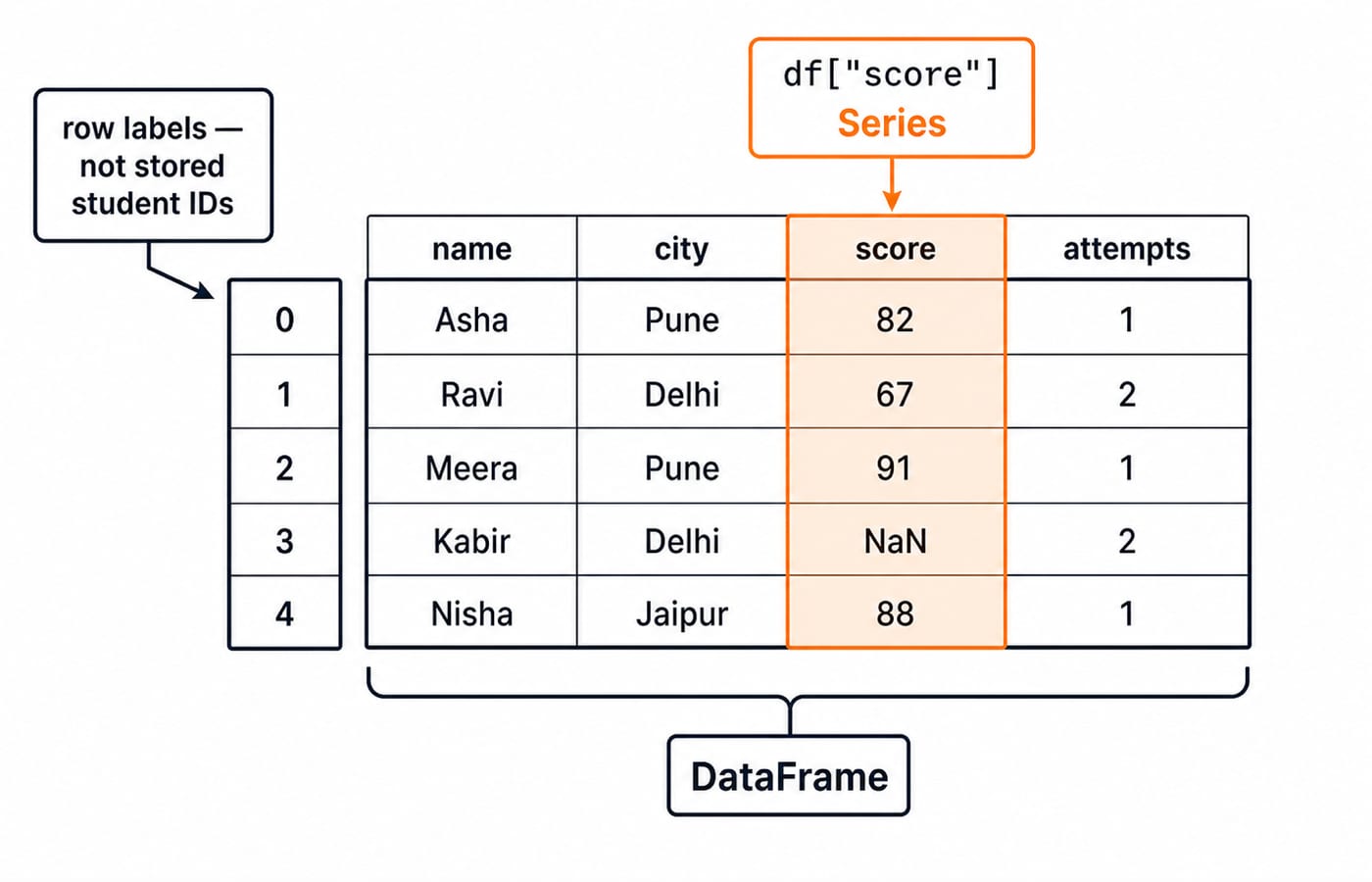
pandas handles labelled, tabular data in Python. A Series is a labelled one-dimensional sequence, such as a score column. A DataFrame is a two-dimensional table whose columns can have different data types.
Install pandas once, then use its conventional pd alias. For broader programming foundations, explore Coding & DSA Courses for Placements.
python -m pip install pandasimport pandas as pdThe fixed table has five rows indexed 0 to 4 and four columns: name, city, score and attempts. Kabir's score is missing. The index labels rows for selection and alignment, but is not automatically a stored student ID.
index | name | city | score | attempts |
|---|---|---|---|---|
0 | Asha | Pune | 82 | 1 |
1 | Ravi | Delhi | 67 | 2 |
2 | Meera | Pune | 91 | 1 |
3 | Kabir | Delhi | NaN | 2 |
4 | Nisha | Jaipur | 88 | 1 |
df["score"] returns a Series. df[["name", "score"]] returns a two-column DataFrame.
Create and inspect the first pandas DataFrame
Run this setup without an external file:
import pandas as pd

students = {
    "name": ["Asha", "Ravi", "Meera", "Kabir", "Nisha"],
    "city": ["Pune", "Delhi", "Pune", "Delhi", "Jaipur"],
    "score": [82, 67, 91, None, 88],
    "attempts": [1, 2, 1, 2, 1],
}

df = pd.DataFrame(students)
Inspect before transforming. df.shape is (5, 4), df.columns.tolist() is ["name", "city", "score", "attempts"], and df.head(3) shows Asha, Ravi and Meera. The missing value makes score floating-point, while attempts stays integer.
A students.csv file could contain the same headers and rows, with Kabir's score field blank. pd.read_csv("students.csv") would load it, but the dictionary is our canonical example.
Select rows and columns with brackets, loc and iloc
Result shape matters. df["name"] is a five-value Series, while df[["name", "score"]] is a 5 by 2 DataFrame.
df.loc[0:2, ["name", "score"]] uses labels, so both ends are included. It returns Asha 82.0, Ravi 67.0 and Meera 91.0. df.iloc[0:3, [0, 2]] uses row positions 0, 1, 2 and column positions 0, 2. The result matches only because the index and column order are unchanged.
Before filling, this Boolean filter returns Asha, Meera and Nisha:
df.loc[df["score"].ge(80), ["name", "score"]]Kabir is excluded because a missing score fails the comparison. Combined masks need parentheses because & joins two complete Boolean Series: (df["score"].ge(80)) & (df["attempts"].eq(1)) selects the same three learners. .loc takes labels or a Boolean mask, while .iloc takes integer positions.
Clean missing data and add a calculated column
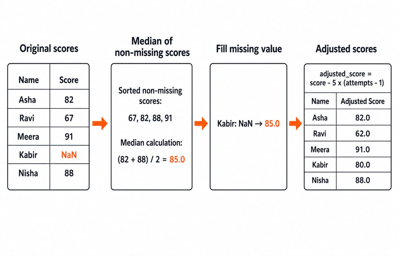
df.isna().sum() reports 1 for score and 0 for the other columns. The sorted non-missing scores are 67, 82, 88, 91, so the median is:
(82 + 88) / 2 = 170 / 2 = 85.0
Fill Kabir's value with that median:
df["score"] = df["score"].fillna(df["score"].median())
df["adjusted_score"] = df["score"] - 5 * (df["attempts"] - 1)
The expression runs across the column and aligns results by row index. No Python loop is needed.
name | score | attempts | adjusted calculation | adjusted_score |
|---|---|---|---|---|
Asha | 82.0 | 1 |
| 82.0 |
Ravi | 67.0 | 2 |
| 62.0 |
Meera | 91.0 | 1 |
| 91.0 |
Kabir | 85.0 | 2 |
| 80.0 |
Nisha | 88.0 | 1 |
| 88.0 |
Median filling is a transparent teaching choice, not a universal rule. First decide whether missing means unknown, not applicable, not attempted or a data-entry fault. That meaning determines whether to use fillna, dropna or a missingness flag.
Group, aggregate, sort and export the cleaned data
Now summarise the cleaned scores by city:
city_summary = (
    df.groupby("city", as_index=False)
      .agg(mean_score=("score", "mean"), students=("name", "count"))
      .sort_values("mean_score", ascending=False)
)
city | mean_score | students |
|---|---|---|
Jaipur | 88.0 | 1 |
Pune | 86.5 | 2 |
Delhi | 76.0 | 2 |
The means are Jaipur 88 / 1 = 88.0, Pune (82 + 91) / 2 = 173 / 2 = 86.5, and Delhi (67 + 85) / 2 = 152 / 2 = 76.0.
df.sort_values(["score", "name"], ascending=[False, True]) orders the table as Meera, Nisha, Kabir, Asha, Ravi. Sorting Algorithms: Complexity and Comparison is a conceptual bridge to ordering and cost, but this pandas call does not guarantee a particular internal algorithm.
Export with df.to_csv("clean_scores.csv", index=False). The argument stops row labels becoming an extra CSV column. SQL Queries and Joins in DBMS offers a related perspective: pandas works in Python memory, while SQL expresses queries to a database system.
Pandas mistakes and how coding questions test them
Chained assignment uses an ambiguous temporary object, so the original table may not change. Update it with df.loc[df["score"].ge(85), "band"] = "high", or create high = df.loc[df["score"].ge(85)].copy() before adding a separate column.
Filtering before inspecting missing data silently removes Kabir. Check with isna() first, then choose the rule. .loc[0:2] includes label 2, while .iloc[0:2] contains only positions 0 and 1.
CSV export without index=False can produce an unwanted column when loaded again, so pass it to keep row labels out. Prefer explicit reassignment over inplace=True chains so every transformation stays visible.
Three useful output-tracing checks are:
After median filling,
df.loc[df["score"].ge(85), "name"].tolist()gives["Meera", "Kabir", "Nisha"].df.iloc[1:4]["name"].tolist()gives["Ravi", "Meera", "Kabir"].df.groupby("city")["score"].mean().idxmax()gives"Jaipur", whose mean is88.0.
These coding and interview checks test shapes, boundaries, missing values and output order.
Pandas basics in short and the next Python step
Recall the pipeline: construct or load, inspect shape and missingness, select, filter, clean with an explicit rule, add vectorised columns, group, sort and export. The key results are shape (5, 4), median 85.0, Kabir's adjusted score 80.0, Pune's mean 86.5, and the order from Meera to Ravi.
For self-practice, change only Ravi's score from 67 to 77. The median stays 85.0; Delhi's mean becomes (77 + 85) / 2 = 162 / 2 = 81.0; Ravi's adjusted score becomes 77 - 5 = 72.0; and the descending score order remains Meera, Nisha, Kabir, Asha, Ravi.
The Python Course: Concepts, MCQs and Coding is a structured next route for Python fundamentals, practice and coding work. First, rerun this example, change one value, and predict the city summary before executing the code.
Keep learning

Python Operators and Expressions: Precedence, Types and Worked Output Traces
Trace Python expressions without guessing. This guide connects operator families, precedence, types, short-circuiting and exact output through worked examples.
Updated 23 Sep 20266 min readPython
CSV Files Explained: Parsing Rules, Worked Records and Exam Traps
Learn why commas and newlines are not always boundaries, trace a quote-aware parser, validate text fields with a schema, and calculate processing costs.
Updated 22 Sep 20265 min readPython

Polymorphism and Dunder Methods in Python: Runnable Examples and Exercises
See how one Python operation supports different types, then build a Vector2D class with readable output, addition, magnitude and equality. Includes runnable code, protocol failures and exercises.
Updated 21 Sep 20265 min readPython

Inheritance in Python: A Practical Tutorial with Examples
Learn how Python classes inherit state and behaviour through runnable examples. Trace super(), overrides, MRO, common mistakes, and three focused exercises.
Updated 19 Sep 20265 min readPython