SQL Queries and Joins in DBMS: sublanguages, joins, and GROUP BY worked out

SQL looks deceptively simple until an exam hands you two tables, a join, and a GROUP BY with a HAVING clause and asks for the exact output rows. Most aspirants lose marks not because SQL is hard, but because they never separate the sublanguages and never hand-trace a join. Let us fix both, and finish with a query you can compute row by row.

SQL sublanguages: DDL, DML, DCL, and TCL

Every SQL statement belongs to one of four sublanguages, and examiners love asking which command sits where.

• DDL (Data Definition Language) defines structure: CREATE, ALTER, DROP, TRUNCATE. These change the schema and auto-commit.

• DML (Data Manipulation Language) changes data: SELECT, INSERT, UPDATE, DELETE. Some texts treat SELECT as a separate DQL (Data Query Language); for exams, remember it as the query verb.

• DCL (Data Control Language) handles permissions: GRANT and REVOKE.

• TCL (Transaction Control Language) bounds transactions: COMMIT, ROLLBACK, SAVEPOINT.

One classic trap: TRUNCATE is DDL and cannot be rolled back on most systems, while DELETE is DML and can. Keep that distinction sharp.

SELECT, WHERE, and DISTINCT

The SELECT clause names the columns; FROM names the table; WHERE filters rows before grouping. A row is kept only if its WHERE predicate evaluates to true, so a NULL comparison (which yields unknown) drops the row.

DISTINCT removes duplicate rows from the result after projection. SELECT DISTINCT dept_id FROM Employees returns each department id once, however many employees share it. Remember that DISTINCT applies to the whole selected row, not a single column, when more than one column is listed.

Joins: inner, outer, and self

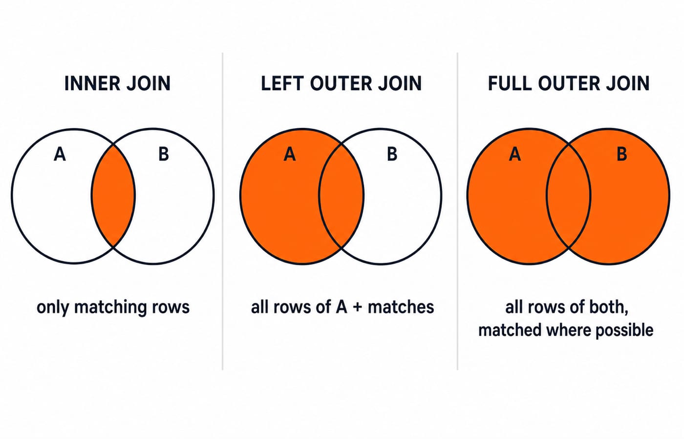
A join combines rows from two tables on a matching condition. This is the heart of relational querying.

• Inner join keeps only rows where the join condition matches in both tables. Unmatched rows vanish.

• Left outer join keeps every row of the left table, padding the right side with NULL where there is no match. Right outer join does the mirror.

• Full outer join keeps unmatched rows from both sides, padding the missing side with NULL.

• Self join joins a table to itself, using two aliases, to relate rows within one table (for example, an employee to their manager in the same table).

[DIAGRAM: Three overlapping-circle set pictures labelled INNER (only the overlap shaded), LEFT OUTER (left circle plus overlap shaded), and FULL OUTER (both circles fully shaded), each captioned with which rows survive.]

GROUP BY, HAVING, and aggregates

Aggregate functions collapse many rows into one value: COUNT, SUM, AVG, MIN, MAX. GROUP BY partitions the rows into groups and computes one aggregate per group. The crucial rule: WHERE filters individual rows before grouping, while HAVING filters whole groups after aggregation. So a condition on COUNT(*) must live in HAVING, never in WHERE.

The logical order of evaluation is worth memorising: FROM and joins first, then WHERE, then GROUP BY, then HAVING, then SELECT projection, and finally ORDER BY. This order explains why a column alias defined in SELECT cannot be used in WHERE.

Nested versus correlated subqueries

A nested (non-correlated) subquery runs once, independently, and hands its result up to the outer query. Example: SELECT name FROM Employees WHERE salary > (SELECT AVG(salary) FROM Employees). The inner average is computed a single time.

A correlated subquery references a column from the outer query, so it re-executes once per outer row. Example: SELECT name FROM Employees e WHERE salary > (SELECT AVG(salary) FROM Employees x WHERE x.dept_id = e.dept_id) compares each employee against their own department average. The e.dept_id reference is what makes it correlated, and what makes it slower.

A worked join with GROUP BY

Take two small tables. Employees holds emp_id, name, dept_id, salary. Departments holds dept_id, dept_name.

Departments: (10, Engineering), (20, Sales), (30, Marketing).

Now run this query:

SELECT d.dept_name, COUNT(*) AS headcount, AVG(e.salary) AS avg_salary FROM Employees e JOIN Departments d ON e.dept_id = d.dept_id GROUP BY d.dept_name HAVING COUNT(*) >= 2;

Step one, the inner join matches every employee to its department by dept_id, giving five joined rows (all employees have a valid dept_id, so none drop).

Step two, GROUP BY d.dept_name forms three groups:

• Engineering: Asha and Ravi. Count is 2, average is (50000 + 70000) / 2 = 60000.

• Sales: Meera and Karan. Count is 2, average is (60000 + 80000) / 2 = 70000.

• Marketing: Sana alone. Count is 1, average is 55000.

Step three, HAVING COUNT(*) >= 2 drops any group with fewer than two rows, so Marketing is removed. The final output is two rows:

That is exactly the trace an examiner expects: join, group, aggregate, then filter groups. If you had wrongly put the count condition in WHERE, the query would error, because WHERE runs before any group exists.

How SQL joins are tested in GATE, NET, and placements

GATE CS asks output-prediction questions: given two small tables and a query with a join plus GROUP BY, HAVING, or a correlated subquery, count the exact rows in the result. Nested-versus-correlated evaluation counts and the difference between a left join and an inner join are recurring numerical and conceptual items. Practise on the solved DBMS SQL queries MCQs, which drill precisely these output-tracing patterns.

UGC NET Computer Science leans conceptual: which sublanguage a command belongs to, the difference between HAVING and WHERE, and what an outer join returns for unmatched rows. Definitions and ordering of clauses are the common targets.

Placement and company tests ask you to write a query live, most often "find the second-highest salary" or "employees earning above their department average", which are correlated-subquery and self-join problems in disguise. Interviewers also probe why one join is faster than another.

To place SQL inside the full relational syllabus, the DBMS learn module sequences querying with the relational model and normalisation, and the wider GATE Guidance by Sanchit Sir course threads it through transactions and indexing.

The short version

Separate the four sublanguages, keep WHERE (rows) apart from HAVING (groups), and know that an inner join drops unmatched rows while an outer join keeps them with NULL padding. Then hand-trace one join with GROUP BY until the row count comes out right on paper. For a structured path through the rest of the exam syllabus, start at the GATE CS exam category. Do that, and SQL output questions turn into guaranteed marks.