Sorting Algorithms Compared: complexity, stability, and the n log n lower bound
Sorting algorithms compared: bubble, insertion, selection, merge, quick and heap sort with best, average and worst time, stability, and the n log n bound.
KnowledgeGate Team
Exam prep & CS education
Updated 14 Jul 20266 min read232 views
Sorting is a fixed part of the algorithms syllabus in GATE, UGC NET and placement tests, and it is where careless aspirants leak marks. The trap is treating six algorithms as six unrelated recipes. They are not. Once you compare them on the same axes, best case, average case, worst case, stability, and memory, the whole topic collapses into one table you can reconstruct from first principles.
Sorting algorithms: what you are actually comparing
Every sorting question is asking about one of five properties. Fix these axes and you can classify any algorithm.
Time complexity in the best, average, and worst case, as a function of the number of elements n.
Stability. A sort is stable if two equal keys keep their original relative order. This matters when you sort records by a secondary key.
In-place. An in-place sort uses only O(1) extra memory beyond the input array.
Comparison versus non-comparison. A comparison sort decides order only by comparing pairs of keys. A non-comparison sort exploits the structure of the keys themselves.
Adaptivity. An adaptive sort runs faster on input that is already nearly sorted.
The elementary sorts: bubble, insertion, selection
These three run in O(n²) on average and are the examiner's warm-up.
Bubble sort repeatedly swaps adjacent out-of-order pairs, letting the largest element "bubble" to the end each pass. With an early-exit flag it detects an already-sorted array in one pass, giving a best case of O(n). It is stable and in-place.
Insertion sort grows a sorted prefix, inserting each new element into its correct place. On nearly-sorted data it is O(n), which makes it the fastest choice for small or almost-ordered arrays. Stable and in-place.
Selection sort repeatedly selects the minimum of the unsorted suffix and swaps it into place. It always does the same work, so best, average, and worst are all O(n²). It is not stable, because a long-distance swap can jump one equal key past another.
Merge sort and quicksort: divide and conquer
Merge sort splits the array in half, sorts each half recursively, and merges the two sorted halves. The merge is the heart of it. Suppose we merge two sorted runs, [2, 5, 8] and [1, 3, 9].
Compare fronts 2 and 1, take 1. Result: [1].
Compare 2 and 3, take 2. Result: [1, 2].
Compare 5 and 3, take 3. Result: [1, 2, 3].
Compare 5 and 9, take 5. Result: [1, 2, 3, 5].
Compare 8 and 9, take 8, then append the leftover 9. Result: [1, 2, 3, 5, 8, 9].
Merging two runs of total length n is O(n), and there are log n levels of splitting, so merge sort is Θ(n log n) in all cases. It is stable but needs O(n) extra memory, so it is not in-place.
Quicksort picks a pivot, partitions the array so smaller elements go left and larger go right, then recurses. Here is a Lomuto partition of A = [8, 2, 3, 6, 7, 1, 5, 4] with pivot 4 (the last element). We keep a boundary index i for the "less than or equal to pivot" region, starting at i = -1, and walk j across the rest of the array.
j = 0: A[0] = 8 > 4, skip.
j = 1: A[1] = 2 ≤ 4, advance i to 0 and swap A[0] with A[1]. Array: [2, 8, 3, 6, 7, 1, 5, 4].
j = 2: A[2] = 3 ≤ 4, advance i to 1 and swap A[1] with A[2]. Array: [2, 3, 8, 6, 7, 1, 5, 4].
j = 3, 4: 6 and 7 both exceed 4, skip.
j = 5: A[5] = 1 ≤ 4, advance i to 2 and swap A[2] with A[5]. Array: [2, 3, 1, 6, 7, 8, 5, 4].
j = 6: A[6] = 5 > 4, skip.
Finally swap the pivot into position i + 1 = 3, giving [2, 3, 1, 4, 7, 8, 5, 6]. The pivot 4 is now in its final sorted slot, with 2, 3 and 1 on its left and 7, 8, 5 and 6 on its right. Quicksort then recurses on those two sides.
![Bar chart of A = [2, 3, 1, 6, 7, 8, 5, 4] before the final Lomuto swap and [2, 3, 1, 4, 7, 8, 5, 6] after it, with the pivot 4 moving from index 7 to index 3.](https://cdn.knowledgegate.ai/blog-assets/blog_asset_1784032298427_d69qnu.jpg)
Quicksort is O(n log n) on average when partitions are balanced, but O(n²) in the worst case, when the pivot is always the smallest or largest element (a sorted array with a fixed end pivot). It is in-place but not stable.
Heap sort
Heap sort builds a max-heap, then repeatedly extracts the maximum to the end of the array. Building the heap is O(n), not O(n log n), and that catches people out: sifting down from the last internal node upwards, only about n/4 nodes can travel one level, n/8 two levels, n/16 three, and the series n/4 + 2(n/8) + 3(n/16) + ... sums to roughly n. Each of the n extractions then costs O(log n), so heap sort is Θ(n log n) in every case, and in-place. It is not stable, because sifting an element down can carry it past an equal key. It is the algorithm that gives you guaranteed n log n without merge sort's extra memory, which is why it is the answer when a question demands worst-case n log n in O(1) space.
The Ω(n log n) comparison lower bound
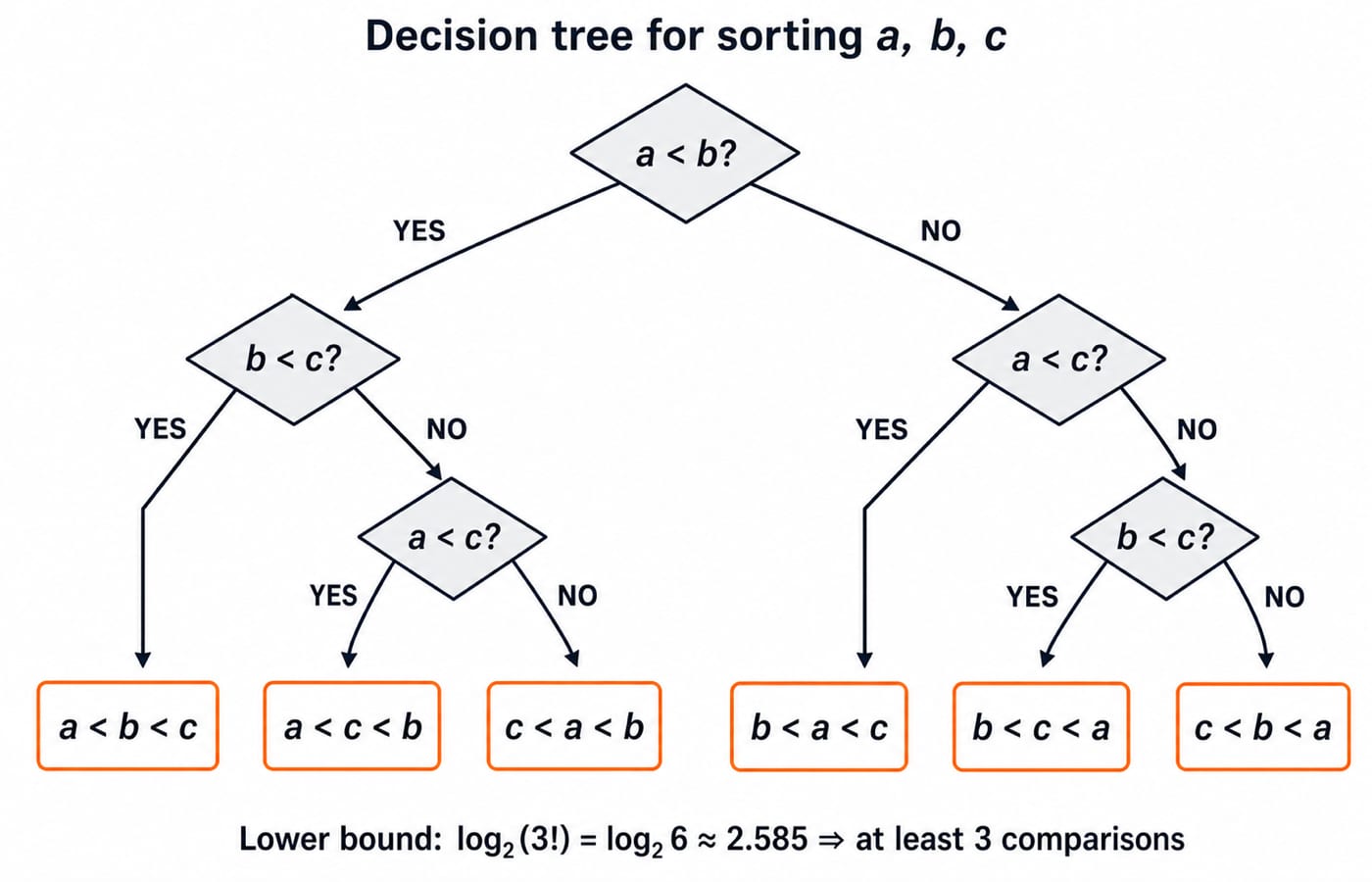
Why can no comparison sort beat n log n? Model any comparison sort as a binary decision tree, where each internal node is one comparison and each leaf is one possible ordering of the input. For n distinct elements there are n! possible orderings, so the tree needs at least n! leaves. A binary tree with n! leaves has height at least log₂(n!), and by Stirling's approximation log₂(n!) is Θ(n log n). The height equals the worst-case number of comparisons, so every comparison sort is Ω(n log n). This is a proof, not a heuristic, and examiners ask it directly.
Non-comparison sorts: counting and radix
If keys are integers in a small range, you can beat the bound because you are no longer only comparing. Counting sort counts occurrences of each key value and reconstructs the array in O(n + k) time, where k is the range of key values. It is stable. Radix sort applies a stable sort (usually counting sort) digit by digit, from least significant to most significant, running in O(d(n + k)) for d-digit keys. These are linear only when k and d are small relative to n, which is exactly the constraint examiners test.
Sorting complexity: the comparison table
Algorithm | Best | Average | Worst | Stable | In-place |
|---|---|---|---|---|---|
Bubble | O(n) | O(n²) | O(n²) | Yes | Yes |
Insertion | O(n) | O(n²) | O(n²) | Yes | Yes |
Selection | O(n²) | O(n²) | O(n²) | No | Yes |
Merge | O(n log n) | O(n log n) | O(n log n) | Yes | No |
Quick | O(n log n) | O(n log n) | O(n²) | No | Yes |
Heap | O(n log n) | O(n log n) | O(n log n) | No | Yes |
How sorting is tested in GATE, NET and placements
GATE CS favours the corner cases: the worst-case input for quicksort, the exact count of comparisons or swaps for a small array, which sorts are stable, and the decision-tree lower-bound argument. A recurring numerical asks you to hand-trace one partition or one merge, so practise both by hand until you can do them without notes. To place sorting inside the wider algorithms syllabus, the Algorithms learn module sequences it with searching and complexity analysis.
UGC NET Computer Science leans conceptual: match an algorithm to its complexity, identify stability, and distinguish comparison from non-comparison sorts. Placement tests ask you to code quicksort or merge sort and reason about when each is preferable, and often connect sorting to later topics like the graph algorithms behind BFS, DFS and shortest paths or the optimisation patterns in dynamic programming.
The short version
Learn the comparison table by understanding, not memory: the O(n²) sorts trade simplicity for speed, merge and heap sort guarantee n log n, quicksort is fast on average but quadratic on a bad pivot, and non-comparison sorts win only when the key range is small. Hand-trace one partition and one merge, then prove the n log n lower bound once. For GATE-depth practice across the whole algorithms syllabus, GATE Guidance by Sanchit Sir sequences these with hundreds of solved questions, and the GATE CS exam category collects the rest of the paper. Do the tracing by hand and sorting becomes guaranteed marks.
Keep learning
Tree Data Structure: Types, Traversals and a Worked BST Example
Build one nine-node binary search tree, classify its shape, trace four traversals, and work through insertion, search, deletion and complexity checks.
Updated 21 Oct 20266 min readDSA & Algorithms
Graphs in Data Structures: Complete Guide with BFS, DFS and Dijkstra Worked Examples
Learn graph terminology, representations and algorithm selection by tracing one unweighted graph with BFS and DFS, then solving a weighted graph with Dijkstra.
Updated 17 Oct 20266 min readDSA & Algorithms

Physical Security and Cryptography Basics: Controls, Keys and Worked Examples
Learn how physical and cryptographic controls work together, then apply them in a four-asset server-room model and a step-by-step toy RSA example.
Updated 13 Oct 20265 min readDSA & Algorithms
Stack Data Structure: Operations, Applications and Worked Examples
Build a stack from its LIFO rule, trace array and linked-list operations, evaluate a postfix expression, and practise recursion, applications, and common traps.
Updated 8 Oct 20265 min readDSA & Algorithms