HPSC PGT Computer Science: Algorithms and Computer Architecture Problems
Learn a two-lane method for Algorithms and Computer Architecture practice, with verified Dijkstra, direct-mapped cache, and pipeline examples.
KnowledgeGate Team
Exam prep & CS education
Updated 6 Aug 20265 min read

Algorithms and Computer Architecture both reward precise state tracking, but their scratch work looks completely different. One follows vertices, keys or subproblems. The other splits addresses, counts cycles and identifies hardware fields. Keeping those two lanes separate on paper, then drilling them together in one timed block, is what turns a solvable question into marks rather than a guess in HPSC PGT Computer Science exam preparation.
Check the HPSC syllabus and corrigenda before building a study list
Open the HPSC document for the exact post and advertisement you are preparing for. Check its title, issue date, post name and every corrigendum. Use the official HPSC Syllabus page as your starting checkpoint, then locate the applicable Scheme & Pattern and Previous Year's Question Papers on the HPSC website.
HPSC does not score Algorithms and Computer Architecture as one section. They pair well for practice because both reward writing the changing state down before you answer. Marks, question counts, sectional timing and negative marking for your post are specified only in the applicable HPSC notice or syllabus. Every numerical here is practice built to teach the method, not a reproduced HPSC paper.
Sort Algorithms questions by the state they change
Problem family | State to write | Check before answering |
|---|---|---|
Sorting and searching | Array plus pass or search interval | Invariant and boundary |
Asymptotic analysis | Operation count or recurrence | Input size and case |
Trees and graphs | Visited set, frontier, distance or parent | Direction, edge weights and source |
Greedy methods | Chosen set plus remaining candidates | Selection rule and feasibility |
Dynamic programming | State definition, base cases and transition | Evaluation order and final cell |
A method name is not a solution. Writing BFS, Dijkstra, merge sort or dynamic programming gives no certainty until you record the changing state and requested output. Learn to compare sorting methods by trace and complexity, not by name alone.
Work an Algorithms example from graph to final distances
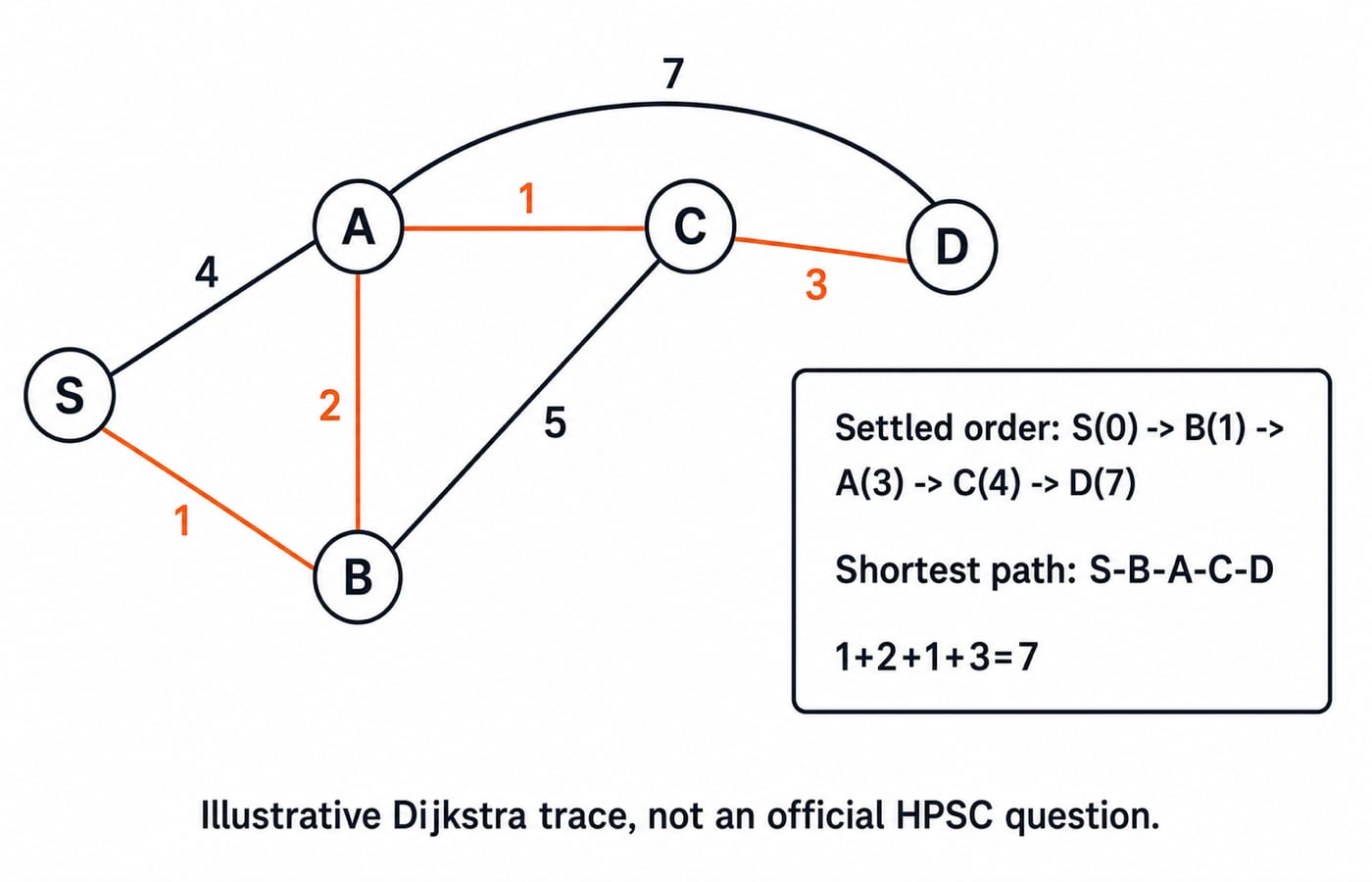
Consider the undirected weighted graph with vertices {S, A, B, C, D} and edges S-A=4, S-B=1, B-A=2, B-C=5, A-C=1, A-D=7, C-D=3. All weights are non-negative, so Dijkstra's algorithm applies from S.
Initialise
d(S)=0; all other distances are infinity.Extract
S: setd(A)=4,d(B)=1.Extract
B: improved(A)=3, setd(C)=6.Extract
A: improved(C)=4, setd(D)=10.Extract
C: improved(D)=7.Extract
Dand finish.
The final distances are S:0, B:1, A:3, C:4, D:7. The shortest route to D is S-B-A-C-D, costing 1+2+1+3=7. Check that extracted tentative distances never decrease, each final value matches its displayed path sum, and no negative edge invalidates the method. With a binary heap, the general bound is O((V+E) log V). That is not the size of this five-vertex instance.
Sort Computer Architecture questions by the fields they expose
Problem family | State or fields to write |
|---|---|
Data representation and arithmetic | Bit width, signed convention and overflow |
Instruction and addressing | Opcode, operands and effective address |
Processor organisation | Register or datapath state and control step |
Cache and memory hierarchy | Address, block, line, tag, index and offset |
Pipelining | Stages, instruction count, clock and stalls |
I/O | Transfer mode, bandwidth and interrupt or polling assumptions |
Write the unit beside every value before calculating. 1 KiB = 1024 bytes, an address may identify a byte rather than a word, and cycles become time only after multiplication by the clock period. Continue with cache mapping and hit-ratio practice.
Work a direct-mapped cache example bit by bit
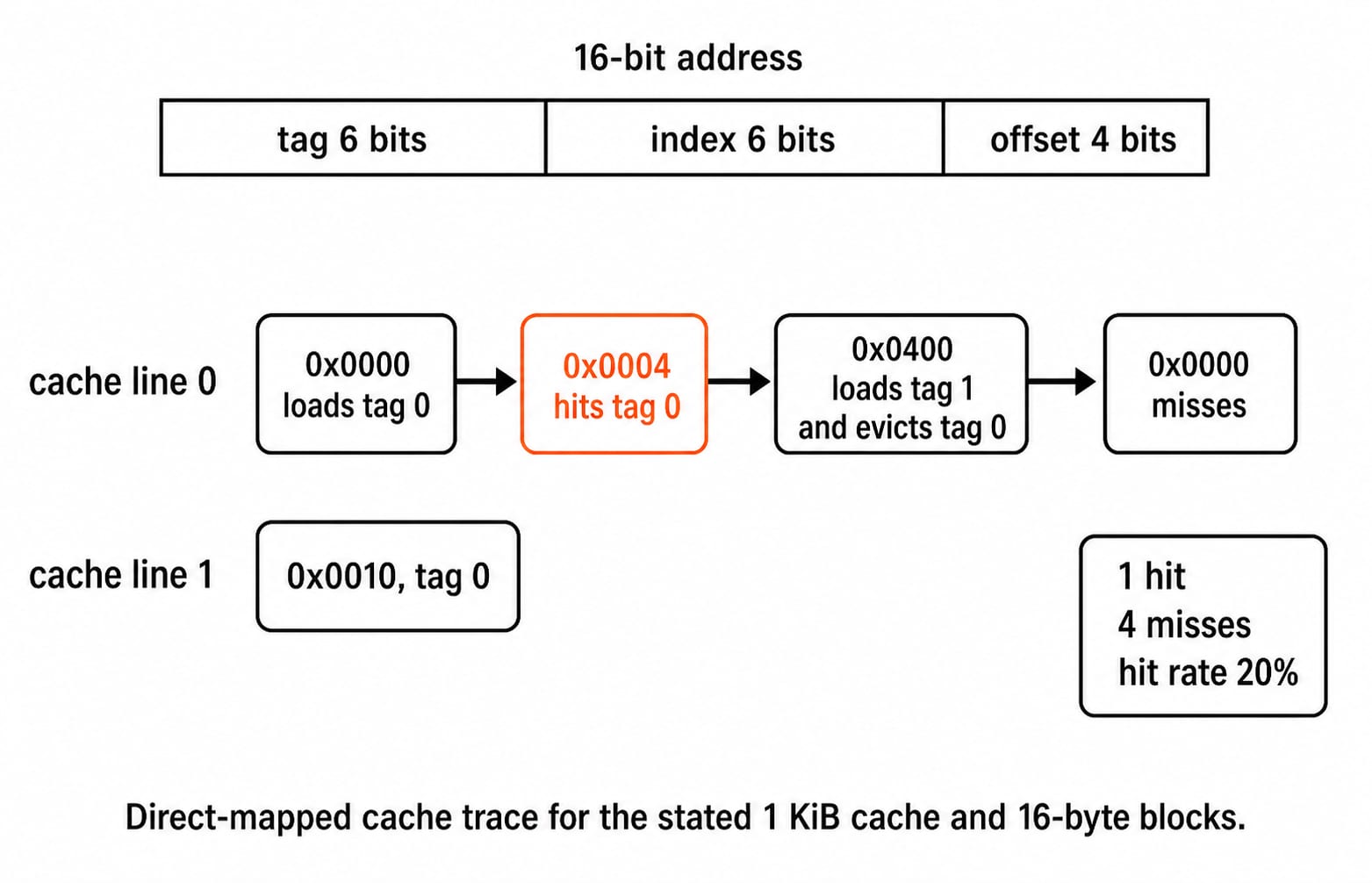
Take a byte-addressable system with 16-bit addresses, a 1 KiB = 1024-byte direct-mapped cache and a 16-byte block. It has 1024/16 = 64 lines. A block needs log2(16) = 4 offset bits, and 64 lines need log2(64) = 6 index bits. The tag therefore uses 16-4-6 = 6 bits.
Starting from an empty cache:
Access | Tag, index, offset | Result |
|---|---|---|
|
| Miss |
|
| Hit in the same 16-byte block |
|
| Miss |
|
| Miss, evicts tag 0 from line 0 |
|
| Miss because of the conflict |
That gives 1 hit, 4 misses, and hit rate 1/5 x 100 = 20%. Check the field width: 6+6+4 = 16 bits. Also, 0x0400 = 1024, so 1024/16 = block 64; its line is 64 mod 64 = 0, and its tag is floor(64/64)=1.
Join the two lanes in a timed mixed drill
Use a 40-minute block: 15 minutes for one Algorithms trace, 15 minutes for one Architecture numerical, 5 minutes to check assumptions and units, and 5 minutes to record the earliest error. After a missed day, resume the same block. Do not double the next session.
Suppose a 5-stage pipeline runs 10 instructions with a 2 ns clock. Ideal cycles are 10+5-1 = 14, one fill of the pipeline for the first instruction plus one cycle each for the remaining nine. Two stalls make the time (14+2) x 2 ns = 32 ns.
A non-pipelined design using 5 cycles per instruction takes 10 x 5 x 2 ns = 100 ns. For these assumptions, speedup is 100/32 = 3.125. Without the stalls the run would take 14 x 2 ns = 28 ns and the speedup would be 100/28 = 3.57, so two lost cycles cost roughly 0.45 of speedup on a run this short. Pipelining improves throughput, not isolated-instruction latency. The HPSC PGT (CS) Test Series runs the same drill against a clock.
Use an error ledger to choose the next revision block
Tag each miss: model for a wrong algorithm or hardware model, state for a lost distance, cache line or stage, arithmetic for a wrong sum, bit count or conversion, or condition for a missed assumption. Record one corrected line and one fresh-value retest.
Each tag has a shape you will recognise. A model miss is reaching for Dijkstra on a graph that carries a negative edge. A state miss is forgetting that extracting A had already lowered d(C) to 4. An arithmetic miss is writing a 5-bit tag because 16-4-6 was done in your head. A condition miss is reading 0x0400 as a word address when the system is byte-addressable.
Next, redo the Dijkstra graph with B-C changed from 5 to 2. Then redo the cache sequence with the fourth access changed from 0x0400 to 0x0020. Build fresh traces instead of memorising earlier answers.
The short version
Confirm the official scope in the HPSC notice, classify by state, label assumptions, check invariants and units, then retest changed values. Use the HPSC PGT Computer Science 2026 complete course for structured revision, or the HPSC test series for timed application.
Keep learning

HPSC PGT vs DSSSB TGT Computer Science: Choose Haryana or Delhi
Use a qualification gate, syllabus-overlap calculation and weighted fit score to decide whether HPSC PGT or DSSSB TGT Computer Science deserves your next study block.
Updated 4 Aug 20266 min readHPSC Teaching
HPSC Teaching CS Weightage: Rank Topics with Four Evidence Signals
Build a defensible HPSC Computer Science revision order without invented percentages. Score syllabus gaps, verified recurrence, prerequisite reach and fresh weakness, then turn the result into a ten-hour week.
Updated 1 Aug 20265 min readHPSC Teaching

HPSC PGT Computer Science Syllabus: Topic Map and Study Order
Turn a flat HPSC PGT Computer Science checklist into six connected preparation lanes. Use the worked school-lab case and balanced diagnostic to decide what to repair next.
Updated 29 Jul 20266 min read75 viewsHPSC Teaching

HPSC Teaching Computer Science: 14-Week Study Plan for Working Aspirants
Use a repeatable 12-hour week to map the official syllabus, diagnose six CS lanes, practise retrieval, review timed sets and finish with focused revision.
Updated 27 Jul 20266 min readHPSC Teaching