

Excel Functions & Charts MCQs: 12 Solved Questions with Explanations
Solve 12 Excel MCQs covering functions, copied references, row and column ranges, SUMIF, and chart vocabulary, with worked explanations.
KnowledgeGate Team
Exam prep & CS education
Updated 7 Nov 20267 min read
Excel MCQs combine function names, cell-reference behaviour, range direction and chart vocabulary. One misplaced $, a reversed range, or confusion between chart type and chart location changes the answer. Build the connected worksheet model in Excel Functions and Charts Explained; then test those ideas against 12 attributed exam questions with answer-by-answer calculations. Choose an option before each explanation, then compare your method and answer. For broader Paper 1 preparation, explore the UGC NET Preparation Courses & Test Series after this focused practice.
1. Build one small worksheet before attempting the Excel MCQs
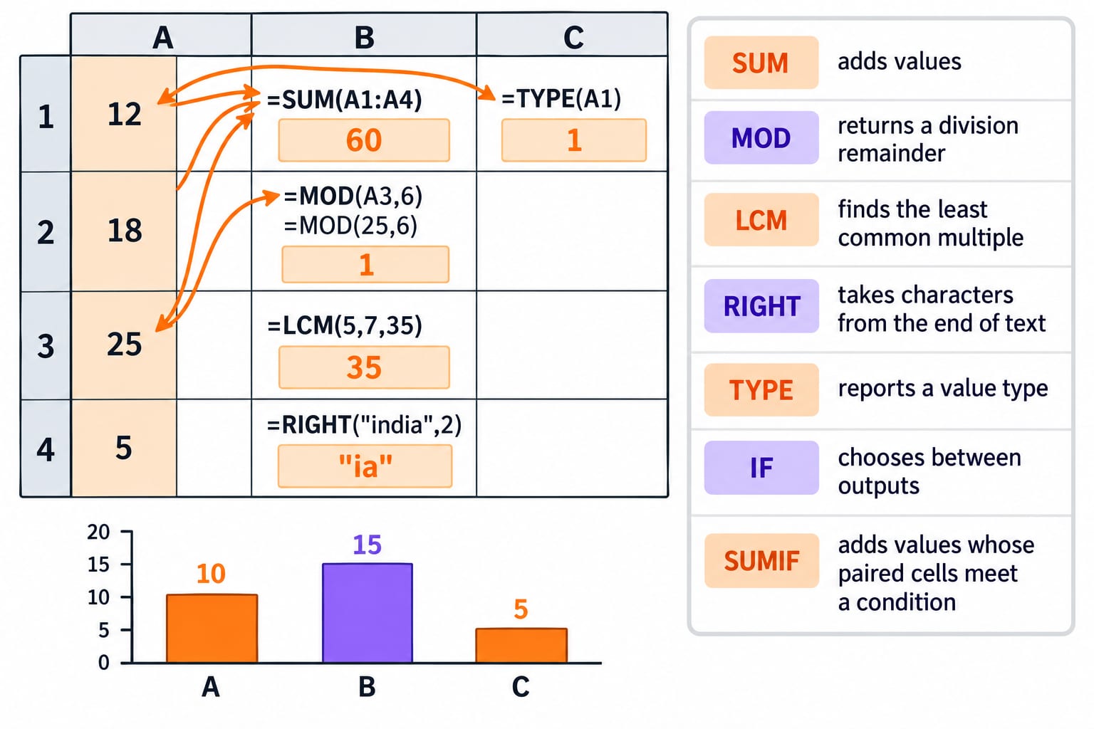
Use this function-purpose map: SUM adds values, MOD returns a division remainder, LCM finds the least common multiple, RIGHT takes characters from the end of text, TYPE reports a value type, IF chooses between outputs, and SUMIF adds values whose paired cells meet a condition. Column is a chart type; embedded describes a chart location.
Use one calibration sheet. Put 12, 18, 25, 5 in A1:A4. Then B1 = SUM(A1:A4) = 60, B2 = MOD(A3,6) = MOD(25,6) = 1, B3 = LCM(5,7,35) = 35, B4 = RIGHT("india",2) = "ia", and C1 = TYPE(A1) = 1 because A1 contains a number. In a table, let A equal 10, B equal 15, and C equal 5; vertical rectangles for those values form a column chart. The rule is simple: identify the requested job, substitute actual values, then evaluate. Use MS Office for CS Teaching Exams when you need the wider concept refresher.
2. Excel MCQs 1-3: recognise functions, AutoSum and remainders
Question 1 (KVS 2023)
__________ is not a basic function of MS Excel.
A. count()
B. sum()
C. min()
D. multiply()
Correct answer: D. multiply().
COUNT, SUM and MIN are built in; multiply() is not. For A1=12 and A2=18, =A1*A2 and =PRODUCT(A1:A2) both give 12×18=216, separating operator from function.
Question 2 (Accenture 2024)
In Microsoft Excel, what is the function of the "AutoSum" button?
A. To automatically correct the selected cell references in a formula
B. To suggest formulas based on the data in adjacent cells
C. To add up the values in the selected range and insert the SUM function automatically
D. To create charts and graphs based on the selected data
Correct answer: C. To add up the values in the selected range and insert the SUM function automatically.
For A1:A4, AutoSum inserts =SUM(A1:A4) and gets 12+18+25+5=60. It neither repairs references nor creates a chart, so C matches.
Question 3 (Accenture 2025)
Which function is used to return the remainder after a number is divided by a divisor in Excel?
A. ROUND ( )
B. FACT ( )
C. MOD ( )
D. DIV ( )
Correct answer: C. MOD ( ).
MOD(25,6) returns 1 because 6×4=24 leaves 1. ROUND changes precision, FACT calculates a factorial, and DIV is not the function.
3. Excel MCQs 4-6: evaluate LCM, RIGHT and TYPE
Question 4 (RSSB 2022)
What will be the output of the following in MS-Excel?
=LCM(5, 7, 35)
A. 70
B. 1225
C. 12
D. 35
Correct answer: D. 35.
LCM(5,7)=35, already divisible by the third input. The LCM remains 35; 1225 merely multiplies inputs.
Question 5 (RSSB 2021)
In MS Excel 2019, what is the result of the formula =RIGHT("india",2)?
A. ia
B. ba
C. aa
D. error
Correct answer: A. ia.
In i n d i a, RIGHT(text,2) takes characters 4 and 5. The result is ia, and valid syntax produces no error.
Question 6 (HTET 2024)
Which Excel function determines whether a cell contains text, a number, a logical value, an array or an error?
A. CELLTYPE
B. TYPE
C. VALUETYPE
D. FORMULATYPE
Correct answer: B. TYPE.
TYPE maps number, text, logical, error and array values to 1, 2, 4, 16 and 64. TYPE(12)=1, TYPE("Excel")=2, TYPE(TRUE)=4, and TYPE(1/0)=16; the other names are not built in.
4. Excel MCQs 7-8: copy references and trace IF row by row
Question 7 (UGC NET January 2026) (question page unavailable; see live Excel Functions & Charts module)
Match the LIST-I with LIST-II in the context of MS-EXCEL
LIST-I (Cell Reference) | LIST-II (Definition and Features) |
|---|---|
A. $D$5 | I. Mixed reference. Row is fixed and column is changeable when fill handle is used |
B. D$5 | II. Mixed reference. Column is fixed and row is changeable when fill handle is used |
C. D5 | III. Absolute reference. Column and row are fixed when fill handle is used |
D. $D5 | IV. Relative reference. Column and row are changeable when fill handle is used |
Choose the correct answer from the options given below:
A. A-III, B-I, C-IV, D-II
B. A-II, B-I, C-IV, D-III
C. A-III, B-IV, C-I, D-II
D. A-IV, B-I, C-III, D-II
Correct answer: A. A-III, B-I, C-IV, D-II.
Move two columns right and two rows down: $D$5 stays fixed, D$5 becomes F$5, D5 becomes F7, and $D5 becomes $D7. A dollar sign fixes the next symbol, giving A-III, B-I, C-IV, D-II.
Question 8 (RSSB 2023)
Consider the following Excel sheet. What will be the output in column E?
Excel data:
Row 1: A = 60 | B = A1 | C = 75 | D = a1 | E = IF(A1=C1,"T","F")
Row 2: A = 70 | B = A2 | C = 70 | D = A2 | E = IF(A2=C2,"T","F")
Row 3: A = 90 | B = A3 | C = 90 | D = A3 | E = IF(B3=D3,"T","F")
A. F F F
B. T T F
C. F T T
D. T T T
Correct answer: C. F T T.
Row 1 compares 60 with 75, giving E1=F. Row 2 compares 70 with 70, giving E2=T. B3 and D3 contain A3, giving E3=T, so the output is F T T.
5. Excel MCQs 9-10: orient ranges correctly and compute SUMIF
Question 9 (RSSB 2023)
Sumati has to calculate the average of a range of cells of a spread sheet. She has to display the average of each row and sum of each column. She also has to display the average of all the rows and columns. Consider the range of cells from A1 to H100. Identify the correct answer which can be used by her.
A.
[for rows = Average (A1 : A100)] [for columns = Sum (A1 : H1)] Copy to all rows and columnB.
[for rows = Average (A1 : H1)] [for columns = Sum (A1 : A100)] Copy to all rows and columnC.
[for rows = Sum (A1 : H1)] [for columns = Average (A1 : H100)] Copy to all rows and columnD.
[for rows = Average (A1 : A100)] [for columns = Average (A1 : H1)] Copy to all rows and column and use it for entire sheet
Correct answer: B. [for rows = Average (A1 : H1)] [for columns = Sum (A1 : A100)] Copy to all rows and column.
A row is horizontal, so A1:H1 with 10,20,30,40,50,60,70,80 averages to 360/8=45. A column is vertical, so the A1:A4 check gives 10+15+20+25=70. This orientation scales to 100 rows, making B correct.
Question 10 (UGC NET August 2024) (question page unavailable; see live Excel Functions & Charts module)
Consider the following snapshot of MS-EXCEL worksheet :
A | B | C | |
|---|---|---|---|
1 | 90 | 70 | |
2 | 60 | 170 | |
3 | 150 | 20 | |
4 | 30 | 110 | |
5 | 50 | 40 | |
6 | 130 | 30 | |
7 |
What will be the value of the cell C1 containing the formula
=SUMIF(A1:A6, ">100", B1:B6)in the above worksheet ?
A. 90
B. 390
C. 50
D. 420
Correct answer: C. 50.
Only A3=150 and A6=130 pass >100. SUMIF adds paired values B3=20 and B6=30, giving 20+30=50. A1=90 fails, despite B1=70.
6. Excel MCQs 11-12: identify a column graph and an embedded chart
Question 11 (RSSB 2023)
Representation of data in a graphical manner is an important feature of Excel. Identify it. Also give the name of the component depicted below –

A. Image, Bar
B. Image, Column
C. Graph, Bar
D. Graph, Column
Correct answer: D. Graph, Column.
The figure presents values graphically, so Graph is first. Rectangles rise vertically over A, B and C at approximately 10, 15 and 5, making columns rather than bars. The pair is Graph, Column.
Question 12 (HTET 2023)
Chart created on worksheet is called as __________.
A. Column chart
B. Embedded chart
C. Resolution chart
D. Bar chart
Correct answer: B. Embedded chart.
A chart inside its source worksheet is embedded. One beside the A=10, B=15, C=5 table on Sheet1 fits. Column and bar are visual types; Resolution chart is not a location term.
7. Excel Functions & Charts traps, score diagnosis and the next practice step
Trap | Questions to revisit |
|---|---|
Invented function name versus valid operator or function | Q1 |
Button versus inserted formula | Q2 |
Evaluate rather than recognise | Q3-Q6 |
Reference and range direction | Q7-Q10 |
Chart type versus chart location | Q11-Q12 |
On retry, allow 45 seconds each for Q1-Q6 and Q12, then 90 seconds each for Q7-Q11, totalling 12 minutes 45 seconds. Label misses name, calculation, reference, range or chart. After 24 hours, rework that category and recompute values.
ICT for Teaching Exams: Fundamentals Explained broadens the ICT foundation. Continue with NTA-UGC-NET Paper - 1 for sequenced Paper 1 preparation.
The short version
Substitute values, track row and column direction, read $ literally, and decide whether chart words describe appearance or location. Verify rather than recognise.
Keep learning

Excel Functions and Charts Explained: Formulas, a Worked Sheet and Exam Traps
Learn how Excel formulas, references and charts work by building one mock-test worksheet from scratch. Every output is calculated and every common trap has a fix.
Updated 19 Oct 20265 min readTeaching Recruitment (Computer Science)

Hashing Basics and Functions MCQs: 12 Solved Questions with Explanations
Attempt 12 solved hashing MCQs, then use the step-by-step solutions to revise functions, collisions, load factor, and operation costs.
Updated 30 Oct 20267 min read98 viewsData Structures MCQs

MS Office Applications for Knowledge of ICT: Worked Word, Excel and PowerPoint Tasks
Choose the right MS Office application, then build a connected Week 3 workbook, report and slide deck with verified calculations and clear task distinctions.
Updated 22 Sep 20266 min readTeaching Recruitment (Computer Science)
IISc Administrative Assistant MS Office: Word, Excel and PowerPoint Workflows
Follow one administrative task from raw figures to a Word summary, an Excel calculation sheet and a three-slide PowerPoint brief. Learn the operations and traps at each step.
Updated 30 Oct 20266 min readIISC Administrative Assistant