Dynamic Programming in Algorithms: Complete Guide with Worked Examples for GATE and Interviews

Dynamic programming is unavoidable for a serious GATE CS or coding interview candidate. Knapsack, longest common subsequence and matrix chain multiplication keep returning, yet memorised solutions fall apart as soon as the examiner changes the instance.

The way out is to understand the state, not memorise code. Dynamic programming rests on two properties: overlapping subproblems and optimal substructure. The 0/1 knapsack recurrence can be solved cell by cell, while standard problems and common traps follow from these ideas.

1. What dynamic programming actually is

A problem becomes a good DP candidate when it has two properties:

1. Overlapping subproblems: the same smaller problem appears repeatedly.

2. Optimal substructure: an optimal answer can be built from optimal answers to smaller states.

This separates DP from divide and conquer. Merge sort's halves are disjoint, so caching one does not help with the other. Fibonacci's fib(n-1) and fib(n-2) overlap.

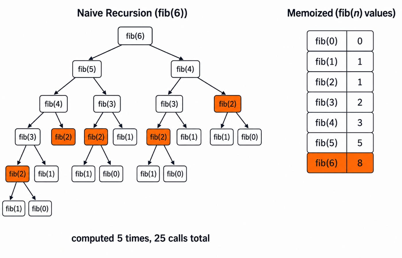
For fib(6) = 8, naive recursion makes 25 function calls and reaches fib(2) five separate times. There are only seven distinct states, fib(0) through fib(6). Remembering each result once changes exponential O(2^n) work to O(n) work.

A useful working definition is: recursion plus a table that remembers answers to subproblems you would otherwise repeat.

If the two properties still feel abstract, Dynamic programming explained builds them from first principles at a gentler pace, with a slower knapsack walkthrough of its own.

2. Memoization vs tabulation

Top-down memoization starts with the recurrence. Check a cache before solving a state, then store the answer. It suits sparse state spaces.

Bottom-up tabulation starts with base cases and fills states in dependency order. It avoids recursion overhead and stack-depth risk. It is clearer for counting operations or reasoning about iteration order.

Both approaches solve the same states at the same asymptotic cost. They produce this Fibonacci table for n = 6:

[0, 1, 1, 2, 3, 5, 8]

Each new entry uses only the previous two, so storing all seven is unnecessary. Two variables reduce space from O(n) to O(1). The same dependency check later lets us compress knapsack from a two-dimensional table to one row.

3. Worked 0/1 knapsack example, cell by cell

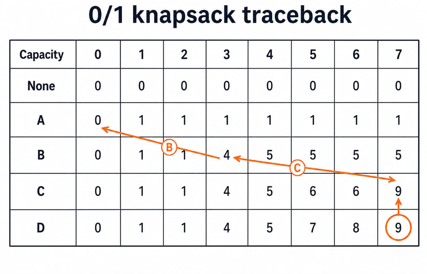
Let capacity W = 7. The items are A (weight 1, value 1), B (3, 4), C (4, 5) and D (5, 7). Define:

dp[i][c] = best value using the first i items within capacity c

The base row is dp[0][c] = 0. If item i is too heavy, copy dp[i-1][c]. Otherwise:

dp[i][c] = max(dp[i-1][c], value_i + dp[i-1][c-weight_i])

The recurrence fills capacities 0 through 7 in each row.

Consider three cells. At dp[2][4], skipping B gives 1, while taking it gives 4 + dp[1][1] = 4 + 1 = 5. At dp[3][5], skipping C gives 5, while taking it gives 5 + dp[2][1] = 5 + 1 = 6. At dp[3][7], skipping C gives 5, while taking it gives 5 + dp[2][3] = 5 + 4 = 9.

Therefore dp[4][7] = 9. To recover the items, compare adjacent rows. Since dp[4][7] = dp[3][7], D is out. Since dp[3][7] != dp[2][7], C is in, and capacity falls to 7 - 4 = 3. Since dp[2][3] != dp[1][3], B is in. The chosen set is {B, C}, with weight 3 + 4 = 7 and value 4 + 5 = 9.

The table takes O(nW) time and O(nW) space. Keeping one row reduces space to O(W), but capacities must be visited from W down to the item's weight.

4. Standard dynamic programming problems

The recurrence changes from problem to problem, but the method does not: define the state, count the states, then measure each transition's cost.

For canonical checks, the LCS of ABCBDAB and BDCABA has length 4, with BCBA as one valid answer. The LIS of [10, 22, 9, 33, 21, 50, 41, 60] has length 5, for example (10, 22, 33, 50, 60). Matrix dimensions (5, 4, 6, 2, 7) have minimum multiplication cost 158.

Each row deserves its own deeper treatment, and the Algorithms course works through each of them in full.

5. Dynamic programming traps

The first trap is using greedy choice without proof. With coins {1, 4, 5} and amount 8, largest-first greedy chooses 5 + 1 + 1 + 1, which is four coins. DP finds 4 + 4, which is two. Greedy needs a valid exchange argument; familiar currency systems can otherwise train the wrong intuition.

Mechanical mistakes are just as costly:

• Wrong base cases, especially confusing dp[0][*] with dp[*][0].

• Forward capacity iteration in compressed 0/1 knapsack. It reuses the current item and silently solves unbounded knapsack instead.

• Off-by-one string indices in LCS.

• Calling O(nW) polynomial in the input length. Knapsack is pseudo-polynomial because W is a numeric value.

The safe complexity rule is simple: number of states multiplied by work per transition.

6. How GATE and interviews test DP

GATE commonly frames DP as recurrence-identification MCQs, table-fill NATs, or complexity questions on LCS and matrix chain multiplication. A table-fill question performs the same knapsack computation with fewer cells exposed. Past papers have also used the (5, 4, 6, 2, 7) matrix-chain instance directly.

Start with past questions because they reveal the actual transformations an examiner expects. Why PYQs beat generic question banks explains that practice order. For syllabus scope and paper-pattern specifics, check the current cycle's official GATE website run by the organising institute. Do not rely on remembered marks or dates.

Interviews test the same idea differently. State the four steps aloud before coding: define the state, write the recurrence, choose the fill order, then optimise space. A correct state explanation is more valuable than rushing into a memorised loop.

7. The short version and next step

Dynamic programming needs overlapping subproblems and optimal substructure. Memoize from the top or tabulate from the bottom. For the worked knapsack, the answer is 9 with items B and C. Learn the standard state shapes and complexities, demand proof before choosing greedy, and practise both cell filling and state definition.

For structured coverage across the Algorithms syllabus, continue with GATE Guidance by Sanchit Sir. Then turn the method into timed topic-wise practice with the GATE Test Series.