Hashing Data Structure: Hash Functions, Collision Resolution and Worked Examples
Trace the same eight keys through separate chaining and linear probing, then learn how tombstones, load factor and rehashing affect correctness and speed.
KnowledgeGate Team
Exam prep & CS education
Updated 24 Sep 20266 min read
Two keys can share a home bucket without being equal, and every collision decision changes the later search path. With h(k) = k mod 11, eight keys produce chain traversals, a wrapped probe cluster and a deletion case where treating a tombstone as empty loses a reachable key. Hash tables solve exact-key lookup problems; cryptographic hashing serves a different purpose. For wider GATE CS preparation, keep the arithmetic methodical from the first insertion.
1. Hash table, hash function, bucket and collision
A hash table is an array of m buckets or slots. A deterministic hash function maps each key to a home index. Let m = 11 and h(k) = k mod 11. Then h(41) = 8 and h(30) = 8. The keys collide because they share a home index. They are different keys, not a duplicate-key update, so a collision rule must place both.
Keep four ideas separate: key, stored value, bucket index and collision rule. A useful hash function remains deterministic while the table configuration is unchanged, returns an index in 0..m-1, runs quickly, and spreads expected keys reasonably. Modulo is not universally good. Patterned keys and an unfortunate m can cluster.
If n keys are stored, the load factor is alpha = n/m. Chaining can hold more than m keys. Open addressing needs a free slot, so it requires alpha < 1.
2. Separate chaining worked from insertion to search
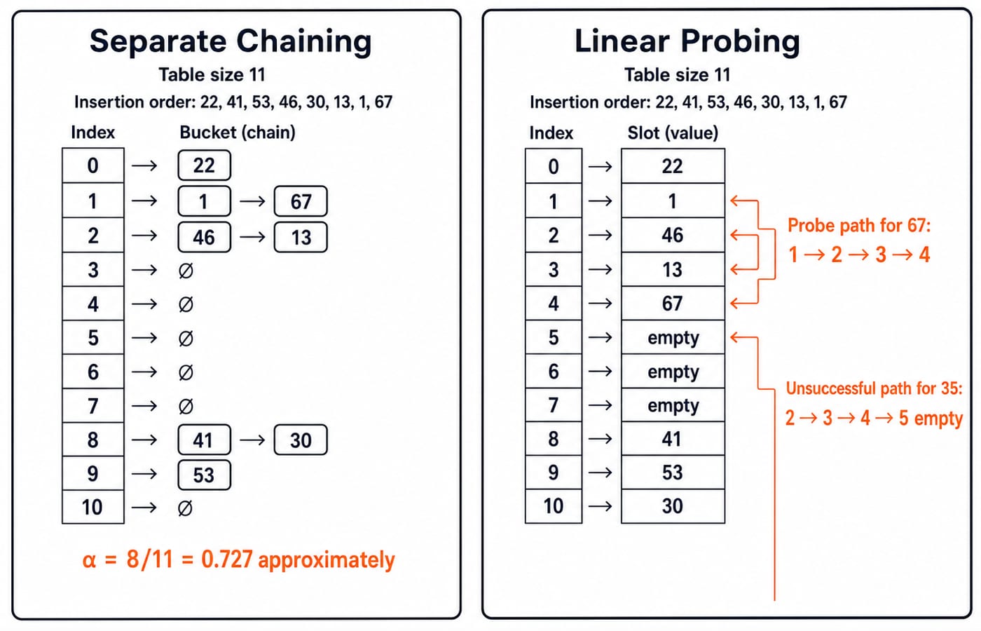
Insert 22, 41, 53, 46, 30, 13, 1, 67 in that order. Their home buckets are:
Key | 22 | 41 | 53 | 46 | 30 | 13 | 1 | 67 |
|---|---|---|---|---|---|---|---|---|
| 0 | 8 | 9 | 2 | 8 | 2 | 1 | 1 |
Append a colliding key to the end of its chain. The final non-empty buckets are:
Bucket | Chain |
|---|---|
0 |
|
1 |
|
2 |
|
8 |
|
9 |
|
Buckets 3, 4, 5, 6, 7, 10 are empty. Here n = 8, m = 11, and alpha = 8/11, approximately 0.727.
To find 13, compute 13 mod 11 = 2, then compare 46 and 13: two key comparisons after hashing. To search unsuccessfully for 35, compute 35 mod 11 = 2, compare 46 and 13, then reach the chain's end.
Appending is this example's policy. Prepending or using another bucket container changes within-chain order, not home buckets. In a map, inserting 41 again should find the equal key and update its value, not add another 41.
3. Linear probing on the same keys
Clear the table and use linear probing:
h_i(k) = (h(k) + i) mod 11, starting with i = 0.
The insertion trace is:
22 -> 041 -> 853 -> 946 -> 230probes8, 9, 10and lands at1013probes2, 3and lands at31 -> 167probes1, 2, 3, 4and lands at4
The final table is:
Slot | 0 | 1 | 2 | 3 | 4 | 5 | 6 | 7 | 8 | 9 | 10 |
|---|---|---|---|---|---|---|---|---|---|---|---|
Key | 22 | 1 | 46 | 13 | 67 | empty | empty | empty | 41 | 53 | 30 |
A successful search for 67 starts at home slot 1 and examines slots 1, 2, 3, 4, so it takes four probes. An unsuccessful search for 35 starts at 2, examines 2, 3, 4, 5, and stops when slot 5 is genuinely empty. It also takes four probes.
Viewed circularly, occupied slots form the run 8, 9, 10, 0, 1, 2, 3, 4. This is primary clustering. Wrapping from 10 to 0 follows directly from modulo arithmetic. Count each occupied probe in order instead of jumping to the eventual slot.
4. Quadratic probing, double hashing, deletion and rehashing
Place 22 at 0, 41 at 8, 53 at 9, and 46 at 2. Now insert 52, whose home is 52 mod 11 = 8.
Linear probing checks
8, 9, 10and places52at10.Quadratic probing,
h_i(k) = (h(k) + i^2) mod 11, checks8, 9, 1and places it at1.Double hashing uses
h1(k) = k mod 11andh2(k) = 1 + (k mod 10). For52, the step is1 + 2 = 3, so it checks8, 0, 3and places the key at3.
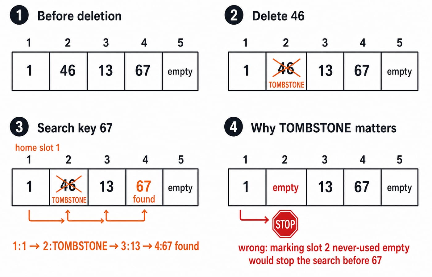
Whichever formula the question states is the one you must follow exactly. In the linear-probing table, delete 46 from slot 2 with a tombstone. Searching for 67 must continue through 1:1, 2:tombstone, 3:13, and 4:67. A never-used empty marker would stop too early. An insertion may reuse a tombstone under its rule.
Resizing rehashes every key. At capacity 23, 30 mod 23 = 7, not old home 8, and alpha = 8/23, approximately 0.348. No threshold suits every implementation.
5. Complexity, load factor and when hashing is the right structure
Operation or event | Separate chaining | Open addressing |
|---|---|---|
Lookup, insert, delete | Expected | Expected |
Worst case |
|
|
Resize |
|
|
With controlled alpha, chaining has expected O(1) cost. Open addressing can too, but probes lengthen as the table fills. Resizing costs O(n), even when insertion is amortised expected O(1) under a growth policy. Hash tables are not always O(1).
Choose hashing for exact-key lookup when order is unnecessary. Use Hashing and collision resolution for a concise choice between chaining and open addressing. For the eight-key calculation, keep the same insertion order across matched chaining and probing tables, count every probe, preserve deletion paths with tombstones, and recompute every index after a resize. Balanced search trees support ordered traversal and range queries; lookup, insert and delete cost O(log n). Not every binary tree is balanced. For repeated ordered output, maintain sorted order instead of forcing it from a hash table.
6. How GATE-style questions and interviews probe hashing
Common practice forms ask you to compute home slots, trace a stated collision rule, count probes, distinguish empty slots from tombstones, calculate alpha, identify primary clustering, or choose an ordered structure. These are practice patterns, not an official-paper guarantee.
In the linear-probing table, where is 30, and how many slots does its search examine? Since h(30) = 8, examine 8:41, 9:53, then 10:30: slot 10, three probes. Searching for 35 may stop at slot 5 because a never-used empty slot proves that no matching key lies farther along that probe sequence. A tombstone instead preserves the sequence after deletion.
The question bank has more than 140 Hashing questions across basic functions, chaining and open addressing. Use Data Structures MCQs for a mixed concept check, or the GATE Test Series for timed practice.
7. Hashing traps that change the answer
Trap | Consequence | Correction |
|---|---|---|
Collision versus duplicate |
| Resolve the collision; update only after equality confirms a duplicate. |
Inconsistent probe formula | Starting at | Write the formula and first three indices. |
No wraparound | A probe from | Apply modulo |
Empty versus tombstone | Clearing slot | Preserve a deletion marker. |
Old-index copy on resize | At capacity | Rehash every key. |
For negative keys, normalise language-specific modulo into 0..m-1. Mutable keys are unsafe if hash-relevant or equality-relevant state can change. Equal keys must produce equal hashes.
8. Short version and the next step
Five points matter: the hash function selects a home bucket; collisions need resolution; chaining groups collisions; open addressing follows an exact probe sequence; and load factor, tombstones and resizing govern correctness and speed. Here chaining stores 46 -> 13 in bucket 2, while linear probing puts 67 at slot 4 after probes 1, 2, 3, 4.
Redraw both tables, then use 67, 1, 13, 30, 46, 53, 41, 22 and predict which representation changes. Continue with GATE Guidance by Sanchit Sir for a structured sequence.
Keep learning
Data Structure for GATE: Syllabus Map, Past-Paper Weightage and Preparation Order
Map the official GATE Data Structure scope, read the two 2026 CS sessions without turning them into a forecast, and follow a verified 48-hour study order.
Updated 23 Sep 20264 min readDSA & Algorithms
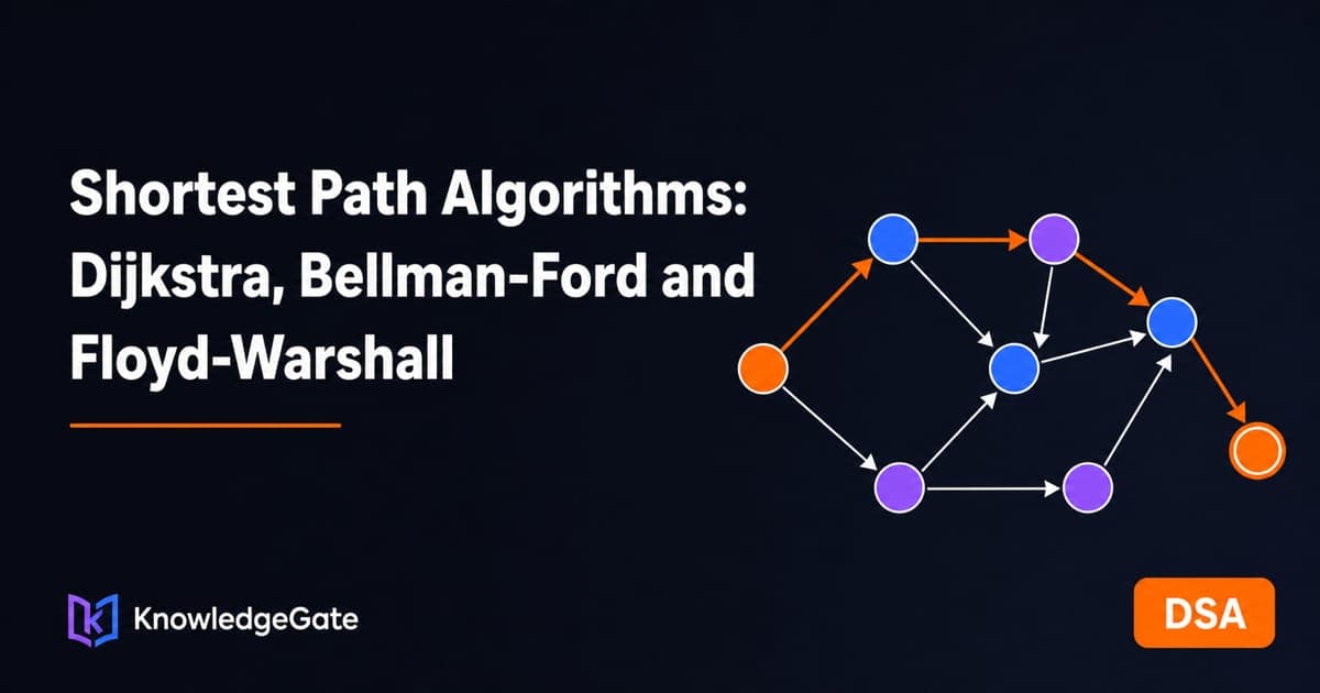
Shortest Path Algorithms: Dijkstra, Bellman-Ford and Floyd-Warshall with Worked Examples for GATE CS
Learn the relaxation idea behind shortest paths, trace three core algorithms by hand, and choose the right method from edge weights and source count.
Updated 21 Sep 20265 min readDSA & Algorithms
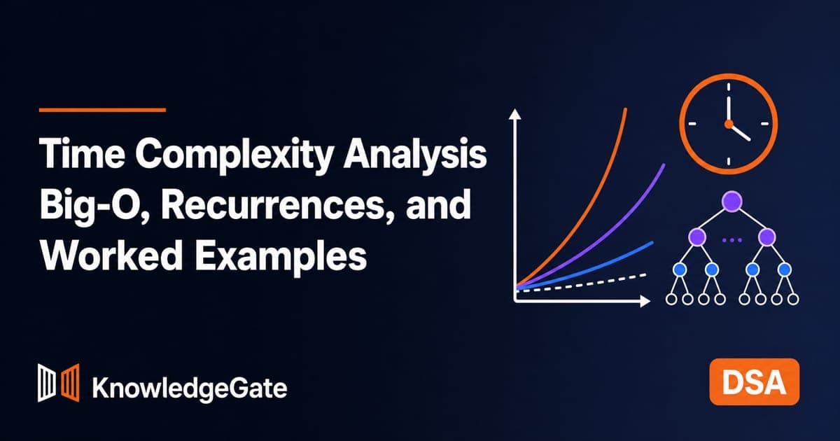
Time Complexity Analysis of Algorithms: Big-O, Recurrences, and Worked Examples for GATE and Interviews
Learn to count operations, compare asymptotic bounds, analyse loops, solve divide-and-conquer recurrences, and explain best and worst cases with confidence.
Updated 20 Sep 20267 min readDSA & Algorithms
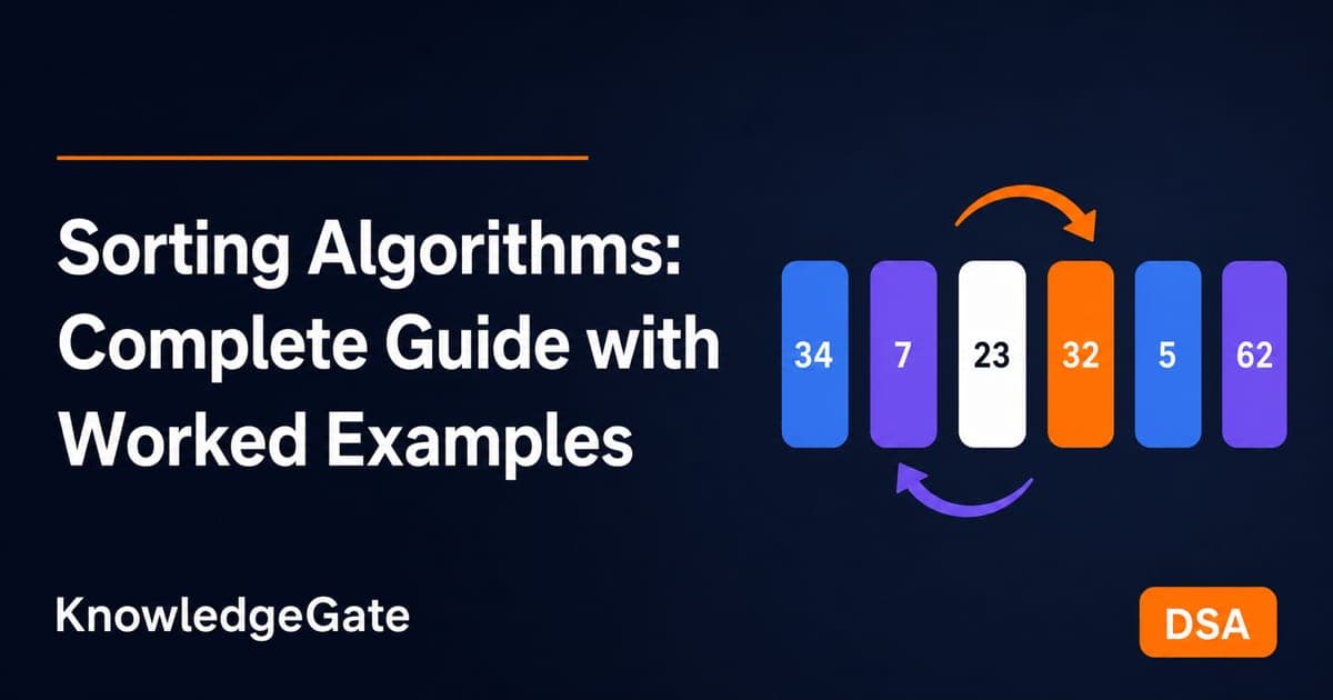
Sorting Algorithms: Complete Guide with Worked Examples for GATE CS and Interviews
Build a reliable sorting toolkit for GATE CS and coding interviews. Compare six core algorithms, follow two worked traces, and learn the traps behind stability, space and pass counts.
Updated 19 Sep 20266 min readDSA & Algorithms