Dynamic Programming Explained: optimal substructure and a worked knapsack
Dynamic programming explained: optimal substructure, overlapping subproblems, memoization vs tabulation, and a fully worked 0/1 knapsack DP table example.
KnowledgeGate Team
Exam prep & CS education
Updated 14 Jul 20265 min read
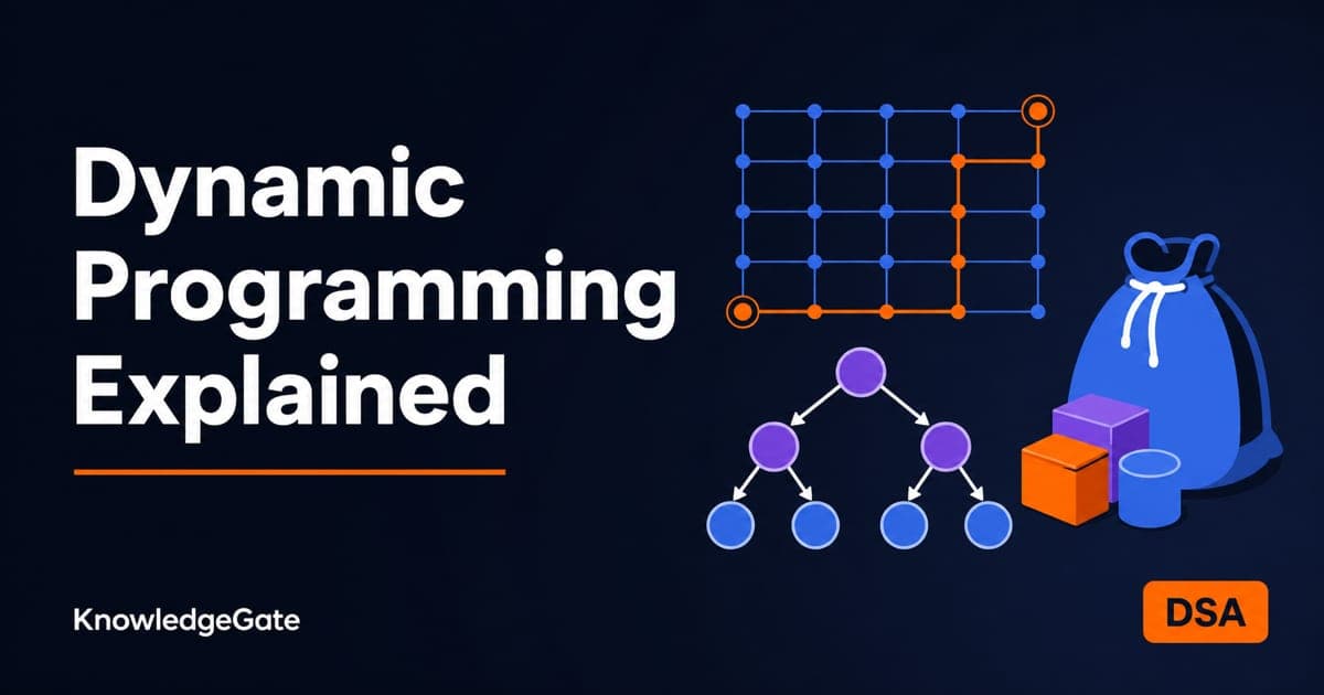
Dynamic programming is the topic that separates aspirants who understand algorithms from those who memorise them. It looks intimidating because it is taught as a bag of tricks. It is not. Dynamic programming is one idea, applied whenever a problem has two specific properties, and once you can spot those properties and fill one table by hand, every DP question becomes mechanical. Those two properties are optimal substructure and overlapping subproblems, and a 0/1 knapsack table is the cleanest place to watch both do their work.
Dynamic programming: optimal substructure and overlapping subproblems
A problem is solvable by dynamic programming when it has both of these:
Optimal substructure. An optimal solution to the whole problem is built from optimal solutions to its subproblems. The shortest path from A to C through B uses the shortest path from A to B.
Overlapping subproblems. The recursive solution solves the same subproblem many times. Computing fib(10) by naive recursion takes 177 calls even though only 11 distinct values are involved, and fib(3) alone gets recomputed 21 times. That repetition is the overlap dynamic programming eliminates.
If subproblems do not overlap, plain divide and conquer is enough. The overlap is what makes storing answers pay off.
Memoization vs tabulation
Dynamic programming stores each subproblem's answer once. There are two ways to do it.
Memoization (top-down). Write the natural recursion, but cache each result the first time you compute it and return the cached value on later calls. It computes only the subproblems you actually reach.
Tabulation (bottom-up). Fill a table starting from the smallest subproblems, so every value you need is already computed when you reach it. No recursion stack, and easy to reason about complexity.
Watch it on that Fibonacci recursion. Add a cache and the 177 calls collapse to 19: fib(10) down to fib(0) is computed once each, 11 stored values in all, and every later request is answered from the cache instead of re-descending. Tabulation reaches the same 11 values from the other end, filling an array left to right from fib(0) = 0 and fib(1) = 1, so fib(k) is already sitting there before anything asks for it.
Both give the same asymptotic time. Tabulation is usually preferred in exams because you can draw the table and trace it.
0/1 knapsack: a fully worked example
The 0/1 knapsack problem: given items with weights and values and a bag of capacity W, choose a subset to maximise total value without exceeding W. Each item is taken whole or not at all. Take four items and capacity W = 5:
Item | Weight | Value |
|---|---|---|
1 | 2 | 3 |
2 | 3 | 4 |
3 | 4 | 5 |
4 | 5 | 6 |
Let dp[i][w] be the best value using the first i items within capacity w. The recurrence: if item i is too heavy for w, dp[i][w] = dp[i−1][w]; otherwise take the better of skipping it or including it, dp[i][w] = max(dp[i−1][w], value(i) + dp[i−1][w − weight(i)]). Fill row by row for capacities 0 to 5.
Items considered | w=0 | w=1 | w=2 | w=3 | w=4 | w=5 |
|---|---|---|---|---|---|---|
none | 0 | 0 | 0 | 0 | 0 | 0 |
item 1 (2,3) | 0 | 0 | 3 | 3 | 3 | 3 |
items 1-2 (add 3,4) | 0 | 0 | 3 | 4 | 4 | 7 |
items 1-3 (add 4,5) | 0 | 0 | 3 | 4 | 5 | 7 |
items 1-4 (add 5,6) | 0 | 0 | 3 | 4 | 5 | 7 |
Read the last cell: dp[4][5] = 7. Trace it back. At w = 5 the value 7 first appears when item 2 is added, from 4 (value of item 2) plus dp[1][2] = 3 (item 1). So the optimal set is items 1 and 2, total weight 2 + 3 = 5, total value 3 + 4 = 7. Note that item 4 alone (weight 5, value 6) is worse, and the table found that automatically.
![Knapsack DP table for four items and capacity 5, with arrows tracing dp[4][5] = 7 back to items 1 and 2.](https://cdn.knowledgegate.ai/blog-assets/blog_asset_1784032178627_jdqdf9.jpg)
The table has (n + 1) rows and (W + 1) columns, and each cell is O(1) work, so 0/1 knapsack is O(nW). More tables of this kind, filled and traced the same way, sit in the Algorithms learn module.
Dynamic programming vs greedy vs divide and conquer
These three strategies are constantly confused, and examiners exploit it.
Divide and conquer splits a problem into independent subproblems: merge sort's two halves never share work, so there is nothing worth storing. That is why the standard sorting algorithms and their complexity are analysed with recurrences rather than tables.
Greedy makes one locally optimal choice at each step and never reconsiders. It is correct only when a greedy choice provably leads to a global optimum, as in fractional knapsack, where you can take a fraction of an item. Greedy fails on 0/1 knapsack.
Dynamic programming considers overlapping subproblems and keeps every partial answer, so it explores the trade-off that greedy skips. It is slower than greedy but correct on the harder problems.
The 0/1 versus fractional knapsack pairing is the cleanest illustration: fractional yields to greedy, 0/1 needs the DP table above.
Complexity: why the table size is the cost
In dynamic programming the running time is the number of distinct subproblems multiplied by the work per subproblem. Knapsack has n times W subproblems at O(1) each, giving O(nW). Longest common subsequence of two strings of lengths m and n has m times n subproblems, giving O(mn). Because W is a number, not the input size in bits, O(nW) is called pseudo-polynomial, a distinction GATE asks about directly.
How dynamic programming is tested in GATE, NET and placements
GATE CS hands you a small instance and asks you to fill or read a DP table: the knapsack value, an LCS length, matrix-chain multiplication cost, or a coin-change count. It also probes the theory, whether a problem has optimal substructure, and the pseudo-polynomial nature of knapsack.
UGC NET Computer Science asks conceptual questions: identify the DP property, distinguish it from greedy, and match a recurrence to its complexity. Placement interviews ask you to code a DP from scratch, and often build on the graph algorithms behind BFS, DFS and shortest paths, since many shortest-path methods are themselves dynamic programming.
The short version
Spot the two properties, optimal substructure and overlapping subproblems, and dynamic programming is on the table. Choose memoization for a natural recursion or tabulation to fill and trace a grid. Practise by hand-filling one knapsack table and back-tracking the chosen items, then contrast it with the greedy fractional version so you know exactly when each applies. For a GATE-depth sequence with hundreds of solved DP problems, GATE Guidance by Sanchit Sir is built for this, and it places dynamic programming alongside the rest of the algorithms paper.
Keep learning
Tree Data Structure: Types, Traversals and a Worked BST Example
Build one nine-node binary search tree, classify its shape, trace four traversals, and work through insertion, search, deletion and complexity checks.
Updated 21 Oct 20266 min readDSA & Algorithms
Graphs in Data Structures: Complete Guide with BFS, DFS and Dijkstra Worked Examples
Learn graph terminology, representations and algorithm selection by tracing one unweighted graph with BFS and DFS, then solving a weighted graph with Dijkstra.
Updated 17 Oct 20266 min readDSA & Algorithms

Physical Security and Cryptography Basics: Controls, Keys and Worked Examples
Learn how physical and cryptographic controls work together, then apply them in a four-asset server-room model and a step-by-step toy RSA example.
Updated 13 Oct 20265 min readDSA & Algorithms
Stack Data Structure: Operations, Applications and Worked Examples
Build a stack from its LIFO rule, trace array and linked-list operations, evaluate a postfix expression, and practise recursion, applications, and common traps.
Updated 8 Oct 20265 min readDSA & Algorithms