UPPSC Computer Science Problem Types: Solve Algorithms, DBMS and OS

You may remember the definitions of insertion sort, 3NF and SJF, yet still lose marks because each numerical needs a different state representation. The cure is a repeatable method for tracing values, writing dependencies and drawing schedules. One four-process dataset, (P1,6), (P2,2), (P3,8) and (P4,3), carries all three: it sorts to P2, P4, P1, P3, splits into two dependency-preserving relations, and schedules to an average waiting time of 4.5. Design and Analysis of Algorithm and Database Management Systems are Computer Paper I headings in the UPPSC Polytechnic Lecturer syllabus, and Operating Systems is a Computer Paper II heading, so the same four records earn marks in both papers. The full nineteen-heading list is in the UPPSC Polytechnic Lecturer CS syllabus topic map.

Convert every stem into state, rule and requested output

Before calculating, write three short lines on the rough sheet:

• State: Copy the values that exist before any operation.

• Rule: Name the operation that is allowed to change the state.

• Output: Write exactly what the question asks you to return.

For algorithms, these become array, loop operation and requested pass. For DBMS, use relation plus dependencies, closure or decomposition, and candidate key or normal form. For OS, use process table, scheduling policy, and timeline or time metric.

"After the second pass" signals a trace. "Determines" and "candidate key" signal dependencies. "Arrival", "burst" and "preemptive" signal a timeline. SJF or 3NF still needs written assumptions.

Algorithm traces: preserve the record while values move

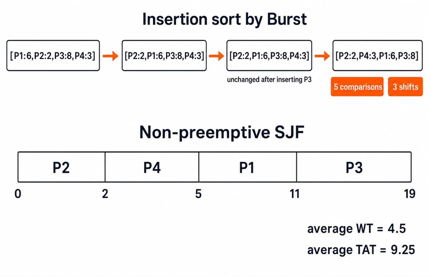
Use records rather than a bare array: (P1,6), (P2,2), (P3,8), (P4,3), with process ID first and burst time second. Ascending insertion sort gives these passes:

Count the work carefully. Inserting P2 uses one burst-value comparison and one shift. Inserting P3 uses one comparison and no shift. Inserting P4 compares against 8, 6 and 2, then shifts two records. The execution therefore has 1 + 1 + 3 = 5 burst-value comparisons and 1 + 0 + 2 = 3 shifts.

These are instance counts, not complexity classes. Insertion sort is O(n^2) worst case and O(n) best case. After pass i, its invariant says positions 0...i are sorted, not that the unprocessed suffix is final. Other methods trade comparisons against shifts differently, and a comparison of sorting algorithms by complexity and stability sets them side by side. Keep each ID attached to its burst, because this order feeds the scheduler.

DBMS dependencies: find the key before naming the normal form

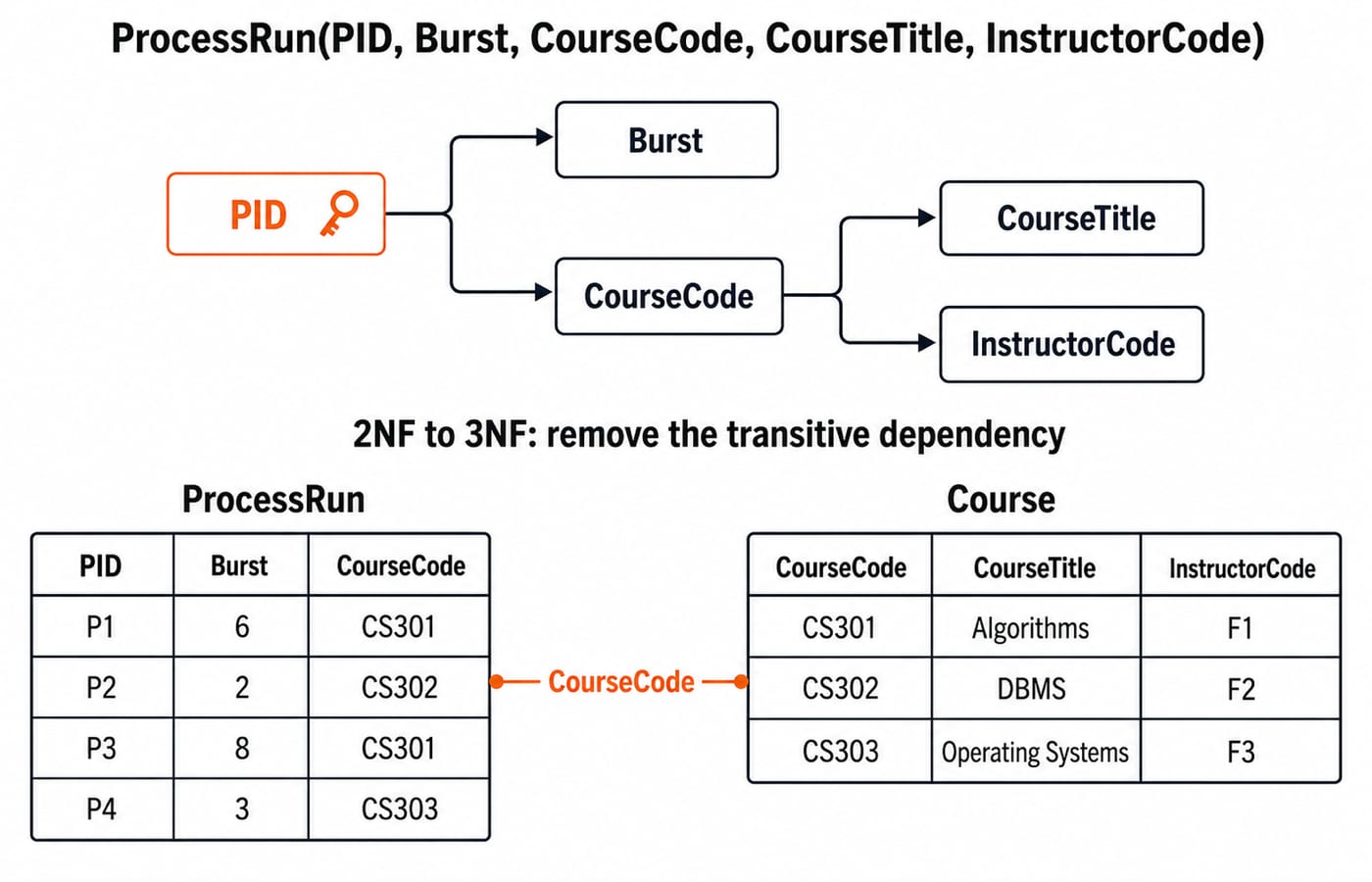
Now store the same records in ProcessRun(PID, Burst, CourseCode, CourseTitle, InstructorCode):

The functional dependencies are:

• PID -> Burst, CourseCode

• CourseCode -> CourseTitle, InstructorCode

Start with {PID}. The first dependency adds Burst and CourseCode; the second adds CourseTitle and InstructorCode. Thus PID+ = {PID, Burst, CourseCode, CourseTitle, InstructorCode}, making PID a candidate key.

The one-attribute key has no proper subset, so there is no partial dependency and the relation is in 2NF. It is not in 3NF because PID -> CourseCode -> CourseTitle, InstructorCode is transitive.

Decompose into ProcessRun(PID, Burst, CourseCode) and Course(CourseCode, CourseTitle, InstructorCode). Each dependency remains checkable inside one component, so the split is dependency-preserving. It is lossless because the common attribute CourseCode is a key of Course. See normalisation from 1NF to BCNF for the broader progression.

OS scheduling: draw the timeline before calculating averages

Assume all processes arrive at time 0, bursts are P1=6, P2=2, P3=8, P4=3, context-switch overhead is zero, and SJF is non-preemptive. Since all are available at time 0, insertion sort gives the valid SJF order P2, P4, P1, P3.

The Gantt chart is 0 | P2 | 2 | P4 | 5 | P1 | 11 | P3 | 19.

Average waiting time is (5 + 0 + 11 + 2) / 4 = 18 / 4 = 4.5. Average turnaround time is (11 + 2 + 19 + 5) / 4 = 37 / 4 = 9.25.

For comparison, FCFS in the original order P1, P2, P3, P4 gives waiting times 0, 6, 8, 16. Its average waiting time is (0 + 6 + 8 + 16) / 4 = 30 / 4 = 7.5. SJF beats it here, 4.5 against 7.5, only because both short jobs were already available at time 0. Move the arrival times and the same burst list can produce a different order and a different average, which is why the timeline is drawn before the averages.

Work the cross-topic chain from one dataset

1. Insertion sort produces P2, P4, P1, P3 from the burst values.

2. Normalisation moves course details into Course while retaining every (PID, Burst, CourseCode) row in ProcessRun.

3. Non-preemptive SJF uses the sorted order and produces average waiting time 4.5 and average turnaround time 9.25.

Sorting produces an order. Normalisation stores records without transitive redundancy. Scheduling turns that order into time metrics. The data is shared, but the correctness tests differ.

Run three checks: the sorted bursts must be 2, 3, 6, 8; joining the decomposed relations on CourseCode must reconstruct all four original rows; and the final Gantt boundary must equal the total burst time, 6 + 2 + 8 + 3 = 19.

Traps that change a correct method into a wrong answer

For algorithms, do not detach PID from its burst value, confuse shifts with comparisons, or quote only asymptotic complexity when the stem asks for a pass. If burst values tie, state the tie rule or stability assumption.

For DBMS, atomic attributes do not prove 3NF. Calculate closure, inspect determinants, and check the common attribute against a component key before calling a decomposition lossless.

For OS, do not sort all bursts globally when arrival times differ, mix preemptive and non-preemptive rules, or average before drawing the timeline. The worked SJF order is valid specifically because every arrival time is 0.

How to practise these forms for the UPPSC CS section

Traces, dependency reasoning and timelines recur across Design and Analysis of Algorithm, Database Management Systems and Operating Systems, so the method survives a change of numbers. Question counts and marks per heading come only from the current notification, so read the advertisement on the official UPPSC website before you budget time by subject.

Use a 30-minute drill: eight minutes for an algorithm pass table, ten for a functional-dependency, key and decomposition problem, ten for a scheduling Gantt chart, and two for the invariant, closure, total-burst and average checks. After a missed day, resume the set instead of doubling it.

The KnowledgeGate question bank holds more than 50,000 practice questions across every subject and exam it covers, so there is no shortage of stems on which to repeat these three forms. Move to timed, exam-scoped sets once each form is reliable untimed.

Short version and next step

Trace algorithms with an invariant, solve DBMS from keys and dependencies, and solve OS from an assumption-labelled timeline. For this example, confirm the sorted bursts 2, 3, 6, 8, reconstruct the original relation through the 3NF join, and finish the schedule at total time 19.

If you still need the subject base underneath these methods, the UPPSC Polytechnic Lecturer 2025 (CS) Course teaches the Paper I and Paper II headings in sequence. If the three methods are already reliable and only timing is missing, the UPPSC Polytechnic Lecturer (CS) Test Series supplies full-length sets.