

Python Performance Profiling: Find and Fix Bottlenecks with timeit and cProfile
A practical Python profiling workflow using timeit, cProfile, and Counter. Follow one bottleneck from a 134.836 ms median to 0.128 ms, with correctness and complexity checks.
KnowledgeGate Team
Exam prep & CS education
Updated 14 Nov 20266 min read
A Python function feels slow, but guessing which line is responsible often leads to cosmetic changes instead of a faster program. A reliable workflow is to establish a baseline, profile a representative workload, find the dominant operation, make one correct change, and measure again. The sample timings are illustrative measurements from one Python 3.14.6 run, so your wall-clock values will vary by machine and Python build.
Python performance profiling starts with the right measurement
Performance is an observed outcome, such as latency, throughput, or peak memory. Profiling explains where execution time or allocations went. The central rule is simple: measure before changing code.
Tool | Best question to ask |
|---|---|
| How long does this small callable take across repeated runs? |
| Which functions account for CPU calls and cumulative time? |
| Where are Python allocations made, and what is the peak traced memory? |
These tools answer different questions. A CPU duration cannot replace a memory measurement, and a profiler duration is not a stable benchmark.
Use this sequence: run a correctness test, choose representative input, record a baseline, profile the workload, change one thing, rerun the correctness test, then remeasure. The Coding & Skill Development Courses category is a broader practice path for applying this loop to real programs.
Python timeit baseline: count repeated values the slow way
The worked input has exactly 10,000 integers. It contains 2,500 distinct values from 0 through 2,499, and each occurs four times.
import timeit
import statistics

values = list(range(2_500)) * 4

def count_slow(values):
    return {x: values.count(x) for x in set(values)}
The expected dictionary has 2,500 keys, with 4 as every count. There is no need to print all the entries to establish that expectation.
Keep input construction outside the timed callable. Repeat the benchmark and convert each result from seconds for ten calls to milliseconds per call:
samples = timeit.repeat(
    lambda: count_slow(values),
    number=10,
    repeat=7,
)
ms_per_call = [seconds * 1_000 / 10 for seconds in samples]
median_ms = statistics.median(ms_per_call)
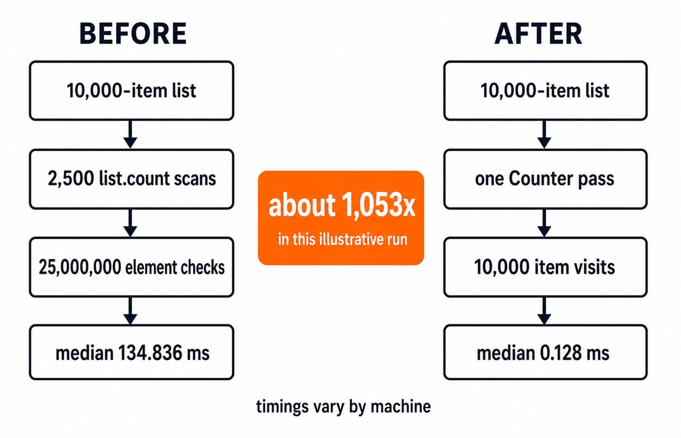
The illustrative samples were 134.629, 134.836, 134.812, 134.859, 134.922, 135.279, 134.625 ms. After sorting, the middle of seven values is 134.836 ms, the median per call. Prefer that repeated median to one unusually fast run. Your CPU and Python build will produce different times, but the dataset and conversion arithmetic remain fixed.
Python cProfile output: find the function consuming the time
Profile one representative function call, not the complete benchmark harness:
import cProfile
import pstats

profiler = cProfile.Profile()
profiler.runcall(count_slow, values)
pstats.Stats(profiler).strip_dirs().sort_stats("cumtime").print_stats(10)
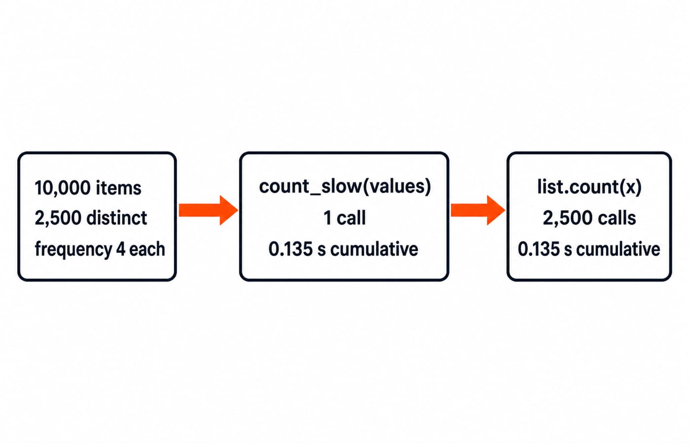
The measured profile reported 2502 function calls in 0.135 seconds. Its load-bearing rows were:
ncalls  tottime  cumtime  function
     1    0.000    0.135  count_slow
  2500    0.135    0.135  list.count
ncalls is the number of calls. tottime is time spent inside that function, excluding subcalls, while cumtime includes its subcalls. Here, list.count was called 2,500 times and accounts for the measured 0.135 s, so it clearly dominates this workload.
cProfile adds instrumentation overhead. Its duration is diagnostic, not the final speed claim. Use timeit for the before-and-after comparison.
Python bottleneck arithmetic: 25,000,000 checks hidden in one line
The comprehension hides repeated work. set(values) produces 2,500 distinct values. For each one, values.count(x) scans all 10,000 list elements. Therefore:
number of scans × elements checked per scan
= 2,500 × 10,000
= 25,000,000 element comparisons
For n input items and u unique values, the repeated counting takes O(n * u) time after building the set. When nearly every item is unique, u approaches n, so the pattern approaches O(n^2).
The Time Complexity and Asymptotic Notation: Big-O tutorial develops this reasoning further. Complexity predicts which operation deserves attention, while profiling confirms whether that cost dominates the actual workload.
Python optimization with Counter: verify first, then claim the speed-up
Counter replaces 2,500 full-list scans with one pass that maintains a count for each key. For Python Collections Module: Counter, defaultdict, deque and namedtuple with Worked Examples, use its counting, query, update and subtraction examples. This profiling experiment uses only the one-pass frequency count as the replacement implementation.
from collections import Counter

def count_fast(values):
    return Counter(values)

assert count_slow(values) == dict(count_fast(values))
That assertion is essential. An optimization is invalid if it changes the result. For this ordinary integer-key workload, Counter visits the 10,000 items once and has expected O(n) time.
Using the same number=10, repeat=7 harness produced 0.129, 0.128, 0.128, 0.128, 0.128, 0.128, 0.128 ms. The median was 0.128 ms per call. Now calculate the comparison explicitly:
speed-up = 134.836 / 0.128 = 1,053.406, about 1,053x
time saved = 134.836 - 0.128 = 134.708 ms per call
lower measured time = (1 - 0.128 / 134.836) × 100 = 99.9051%
These figures describe this illustrative run, not a portable performance guarantee.
Python profiling traps that can produce a false win
Several common mistakes make an optimization look better than it is:
Timing setup or I/O: Input creation, file access, or network waits can hide the function's CPU cost. Move setup outside the timed callable and isolate the work you mean to compare.
Comparing different outputs: A wrong implementation can appear faster because it does less. Assert result equivalence before discussing speed.
Trusting one run: Scheduler noise can distort one measurement. Repeat the benchmark and report the median.
Comparing profiler time with benchmark time:
cProfileadds overhead. Use its call data to locate a hotspot, then use the sametimeitharness for both implementations.Optimizing an irrelevant microbenchmark: A tiny function may improve while total application latency does not. Profile the representative full path first, then benchmark the isolated hotspot.
Do not apply an optimization merely because it wins here. For tiny inputs or code outside a hot path, clear simple code may matter more. If memory growth is the complaint, use tracemalloc snapshots instead of inferring memory behaviour from CPU timings.
How Python performance profiling is tested in interviews and code reviews
Treat the worked input as a miniature interview prompt. A strong answer identifies n = 10,000 and u = 2,500, derives 2,500 × 10,000 = 25,000,000 comparisons, notices the 2,500 list.count calls, proposes Counter, and proves equivalent output before discussing speed.
It also states the measurement question, complexity, harness, and workload assumptions. A weak answer says that one syntax form is always faster, or quotes a time without specifying the input and benchmark setup. This approach reflects general interview and code-review practice rather than any one company or exam process.
DSA Using Python is the relevant next step if you need more practice connecting implementation choices, complexity, and interview-style problem solving.
Python performance profiling: the short version and next step
Use this five-step checklist:
Reproduce the performance problem on representative input.
Choose the metric that matches the complaint.
Establish a repeated baseline.
Profile to locate the dominant cost.
Change one thing, verify the output, and remeasure.
The worked speed-up came from removing 2,500 full-list scans, not from a cosmetic syntax change.
Now try three precise exercises. First, use list(range(5_000)) * 2; predict 5,000 × 10,000 = 50,000,000 comparisons for the slow method before timing it. Second, use list(range(100)) * 100 and explain how u = 100 changes the cost. Third, call tracemalloc.get_traced_memory() around each function and report current and peak traced bytes without claiming that traced Python allocations represent all process memory.
Beginners who need the language foundation can start with Python Course: Concepts, MCQs & Coding. If you are already comfortable with Python syntax, complete the exercises on your own machine and check whether the same hotspot appears.
Keep learning
Python Dictionaries Explained: Keys, Methods, Worked Examples and Exam Traps
Learn how Python dictionaries store, retrieve and mutate values. Trace a complete frequency counter, then practise the membership, aliasing and duplicate-key traps that make output questions tricky.
Updated 18 Nov 20265 min readPython

Python Conditional Statements Explained: if, elif, else, Nested Logic and Worked Examples
Learn a reliable way to trace Python branches, from Boolean expressions and short-circuiting to nested decisions, truthiness, boundary checks, and a complete scholarship classifier.
Updated 17 Nov 20266 min readPython
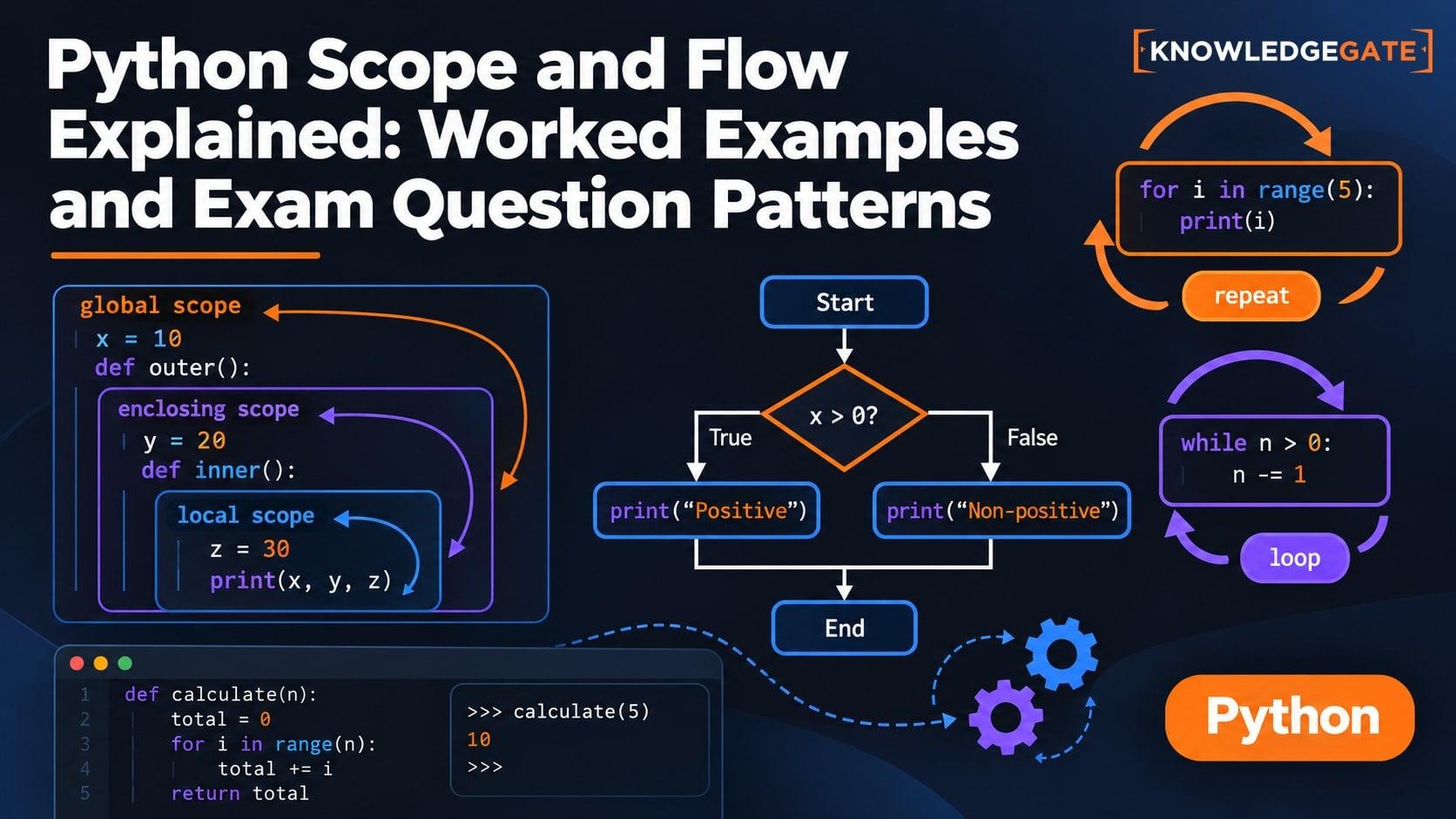
Python Scope and Flow Explained: Worked Examples and Exam Question Patterns
Learn to separate Python name resolution from execution order with a nested-function trace, an UnboundLocalError repair, module examples, and exam-style checks.
Updated 16 Nov 20266 min readPython

Asyncio in Python: Event Loops, Coroutines and Runnable Examples
Build a clear mental model of Python's event loop, then run two dependency-free examples covering concurrent waits, result ordering, timeouts and cleanup.
Updated 15 Nov 20266 min readPython