Time complexity and asymptotic notation: Big-O, Theta and Omega explained
Time complexity and asymptotic notation explained: Big-O, Theta and Omega, growth-rate ordering, analysing loops and recursion, and the Master Theorem.
KnowledgeGate Team
Exam prep & CS education
Updated 16 Jul 20266 min read66 views
Every other algorithm topic leans on this one. Before you can compare sorting methods, reason about a graph traversal, or defend a design in an interview, you need a precise way to say how an algorithm's running time grows with its input. Asymptotic notation is that language, and time-complexity analysis is the skill of reading it off code. The three symbols are short to state exactly, the growth ladder is short to memorise, and loops and recurrences turn into bounds by rule; once those three are solid, every later algorithm question gets easier.
Related reading: asymptotic notation MCQs and loop and recurrence analysis.
Why asymptotic analysis, not a stopwatch
An algorithm's actual running time depends on the machine, the compiler, and the input. To compare algorithms fairly, we ignore constant factors and low-order terms and ask only how the running time scales as the input size n grows large. A method that does 3n² + 5n + 100 operations and one that does n² operations are treated as the same order, n², because for large n the n² term dominates everything else. This is what "asymptotic" means: the behaviour in the limit, where the shape of the growth, not the constants, decides the winner.
Big-O, Omega and Theta: the exact definitions
The three notations bound a function f(n), the operation count, by a simpler function g(n).
Big-O (upper bound). f(n) = O(g(n)) if there exist positive constants c and n₀ such that f(n) ≤ c·g(n) for all n ≥ n₀. It says f grows no faster than g. This is the one people mean by "the complexity", because a worst-case ceiling is what you usually want to guarantee.
Big-Omega (lower bound). f(n) = Ω(g(n)) if there exist positive constants c and n₀ such that f(n) ≥ c·g(n) for all n ≥ n₀. It says f grows at least as fast as g, a floor on the running time.
Big-Theta (tight bound). f(n) = Θ(g(n)) if f is both O(g(n)) and Ω(g(n)), so it is sandwiched: c₁·g(n) ≤ f(n) ≤ c₂·g(n). Theta is the honest description, an exact growth rate rather than just a ceiling or floor.
A common exam point: it is correct but weak to say linear search is O(n²), because O is only an upper bound and n grows no faster than n². The tight statement is Θ(n). Reach for Theta when you can prove both sides.
Best, average and worst case
Complexity also depends on which input of size n you get, and the three cases must not be confused with the three notations above.
Worst case is the maximum time over all inputs of size n, the guarantee you can promise. Quicksort's worst case is Θ(n²).
Best case is the minimum, often not useful on its own. Quicksort's best case is Θ(n log n).
Average case is the expected time over a distribution of inputs. Quicksort's average is Θ(n log n), which is why it is fast in practice despite the quadratic worst case.
Any of the three notations can describe any of the three cases; they are independent axes. "Worst-case O(n log n)" and "best-case Ω(n)" are both meaningful. The same three cases separate the standard sorting methods from one another, worked side by side in sorting algorithms: comparison and complexity.
Growth-rate ordering
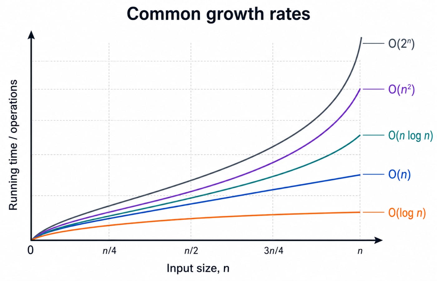
Knowing which function beats which, for large n, lets you rank algorithms at a glance. From slowest-growing (best) to fastest-growing (worst):
O(1) < O(log n) < O(√n) < O(n) < O(n log n) < O(n²) < O(n³) < O(2ⁿ) < O(n!)
Constant time never depends on n; logarithmic time is what halving the problem each step buys you (binary search); linearithmic n log n is the sorting barrier for comparison sorts; polynomial n², n³ come from nested loops; and exponential 2ⁿ and factorial n! signal brute force over all subsets or permutations, which is intractable beyond small n. Memorise this ladder; a large share of quick questions is just placing an expression on it.
Analysing loops and recursion
Turning code into a bound follows a few mechanical rules.
A single loop running n times is O(n). Two nested loops each to n give O(n²); k nested loops give O(nᵏ).
A loop whose bound depends on the outer index (i from 1 to n, j from 1 to i) runs 1 + 2 + ... + n = n(n+1)/2 times. Halving the work does not change the order: triangular nesting is still Θ(n²), not Θ(n).
A loop where the index multiplies or divides by a constant each step (
i = i * 2) runs O(log n) times, because it takes about log₂ n doublings to reach n.Sequential blocks add, so the largest dominates: an O(n) block then an O(n²) block is O(n²).
Recursion is captured by a recurrence relation. Merge sort splits into two halves and does linear merging, giving T(n) = 2T(n/2) + n.
The Master Theorem, with worked cases
The Master Theorem solves divide-and-conquer recurrences of the form T(n) = a·T(n/b) + f(n), where a ≥ 1 subproblems each of size n/b are solved and f(n) is the cost to split and combine. Compare f(n) against n raised to log_b(a):
If f(n) grows slower than n^(log_b a), the leaves dominate: T(n) = Θ(n^(log_b a)).
If f(n) is the same order as n^(log_b a), every level costs the same: T(n) = Θ(n^(log_b a)·log n).
If f(n) grows faster (and a regularity condition holds), the top level dominates: T(n) = Θ(f(n)).
Three standard recurrences, with the comparison worked out in full:
Recurrence | a, b, f(n) | n^(log_b a) | Result |
|---|---|---|---|
T(n) = 2T(n/2) + n | 2, 2, n | n¹ = n | Case 2: Θ(n log n) |
T(n) = 4T(n/2) + n | 4, 2, n | n² | Case 1: Θ(n²) |
T(n) = T(n/2) + 1 | 1, 2, 1 | n⁰ = 1 | Case 2: Θ(log n) |
The first is merge sort, confirming its Θ(n log n). The third is binary search, confirming its Θ(log n). Note the Master Theorem does not apply to every recurrence: T(n) = T(n − 1) + n, for instance, is not in divide-and-conquer form and is solved by expansion to Θ(n²). More solved recurrences of both kinds, in-form and out-of-form, sit in the Algorithms learn module.
How this topic is tested
GATE CS is dense with these questions. Expect to place an expression on the growth ladder, pick the tight Θ bound for a code snippet, solve a recurrence by the Master Theorem or by expansion, or judge a true/false claim about O versus Ω versus Θ. Analysing a nested-loop fragment for its exact complexity is a perennial. Because every other algorithm answer depends on it, this is the highest-leverage topic in the paper, and KnowledgeGate's question bank carries over 170 questions on time-complexity analysis and about 130 on algorithm analysis, so the drill material is deep.
Placement interviews open with it: "what is the time and space complexity of your solution" follows almost every coding question, and you are expected to derive it live from the loops and recursion you just wrote.
The short version
Big-O is an upper bound, Omega a lower bound, and Theta a tight bound; use Theta whenever you can prove both sides. Keep the growth-rate ladder in memory, read loops and recursion into bounds by the mechanical rules, and solve divide-and-conquer recurrences with the Master Theorem's three cases. This is the spine the rest of the algorithms syllabus hangs on.
For a GATE-depth sequence built on this foundation, GATE Guidance by Sanchit Sir is made for it, and placement aspirants can start from the CS Fundamentals category.
Solve one recurrence three ways and rank one set of expressions on the growth ladder, and every later algorithm question inherits the clarity.
Keep learning
Tree Data Structure: Types, Traversals and a Worked BST Example
Build one nine-node binary search tree, classify its shape, trace four traversals, and work through insertion, search, deletion and complexity checks.
Updated 21 Oct 20266 min readDSA & Algorithms
Graphs in Data Structures: Complete Guide with BFS, DFS and Dijkstra Worked Examples
Learn graph terminology, representations and algorithm selection by tracing one unweighted graph with BFS and DFS, then solving a weighted graph with Dijkstra.
Updated 17 Oct 20266 min readDSA & Algorithms

Physical Security and Cryptography Basics: Controls, Keys and Worked Examples
Learn how physical and cryptographic controls work together, then apply them in a four-asset server-room model and a step-by-step toy RSA example.
Updated 13 Oct 20265 min readDSA & Algorithms
Stack Data Structure: Operations, Applications and Worked Examples
Build a stack from its LIFO rule, trace array and linked-list operations, evaluate a postfix expression, and practise recursion, applications, and common traps.
Updated 8 Oct 20265 min readDSA & Algorithms