NumPy Basics in Python: Arrays, Indexing and Broadcasting with Worked Examples

Python lists are familiar, but numerical work gets awkward when every element needs the same calculation or each row and column needs separate handling. A two-row marks array has shape (2, 3), one int32 dtype and three subject columns; a (3,) bonus vector broadcasts across both rows. If the Python syntax itself feels unfamiliar, begin with Python Course: Concepts, MCQs & Coding.

1. NumPy basics start with one array

If NumPy is not installed, use python -m pip install numpy, then import it with the standard alias. NumPy's official beginner guide covers installation and calls the main array type an ndarray.

import numpy as np

marks = np.array(
    [[72, 80, 65],
     [90, 88, 94]],
    dtype=np.int32
)

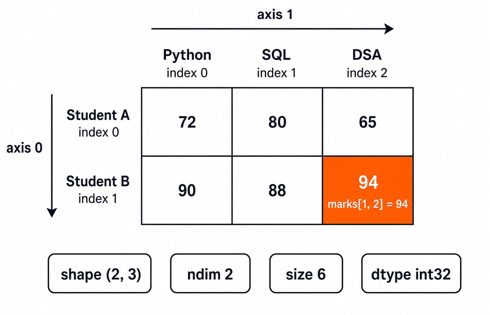
Row 0 is Student A and row 1 is Student B. Columns 0, 1 and 2 are Python, SQL and DSA. This is a two-dimensional array with one declared element type, int32. A nested Python list can instead contain elements of unrelated types.

The distinction matters in arithmetic. [1, 2, 3] + [10, 20, 30] concatenates lists into [1, 2, 3, 10, 20, 30]. With arrays, np.array([1, 2, 3]) + np.array([10, 20, 30]) performs element-wise addition and gives [11, 22, 33]. The Coding & DSA Courses for Placements path places this numerical idea within broader coding preparation.

2. Read shape, dimensions, size, dtype and axes

For this dataset, marks.shape == (2, 3), marks.ndim == 2, marks.size == 6, and marks.dtype == np.dtype('int32'). Shape means two rows by three columns, ndim reports two axes, and size counts all six stored elements. The declared dtype keeps the example independent of machine defaults. NumPy owns homogeneous numerical arrays, broadcasting and axis operations; the earlier Pandas Basics in Python owns labelled, mixed-type tables, missing-value cleaning and group-by analysis.

Axis 0 runs down the student rows. A reduction on it leaves one result per subject. Axis 1 runs across the subject columns and leaves one result per student. When the array is printed row by row, the last index, the column index, changes fastest.

3. Index, slice and filter without losing shape

marks[1, 2] returns the scalar 94. marks[-1, -1] reaches the same scalar from the end. In contrast, marks[0] returns the one-dimensional array [72, 80, 65] with shape (3,).

The slice marks[:, 1:] means all rows, then columns from index 1 onward. It keeps SQL and DSA and produces:

[[80, 65],
 [88, 94]]

Its shape is (2, 2). The Boolean expression marks >= 85 creates a mask of the original shape. Applying it as marks[marks >= 85] returns [90, 88, 94], a one-dimensional result in row-major encounter order.

A correction can also be expressed without mutating the source:

corrected = np.where(marks < 70, 70, marks)
corrected
array([[72, 80, 70],
       [90, 88, 94]], dtype=int32)

np.where returns a new result here. The original DSA mark 65 in marks remains unchanged.

4. Use vectorised arithmetic and broadcasting

Now add a fixed bonus for Python, SQL and DSA:

bonus = np.array([3, 0, 2], dtype=np.int32)
adjusted = marks + bonus

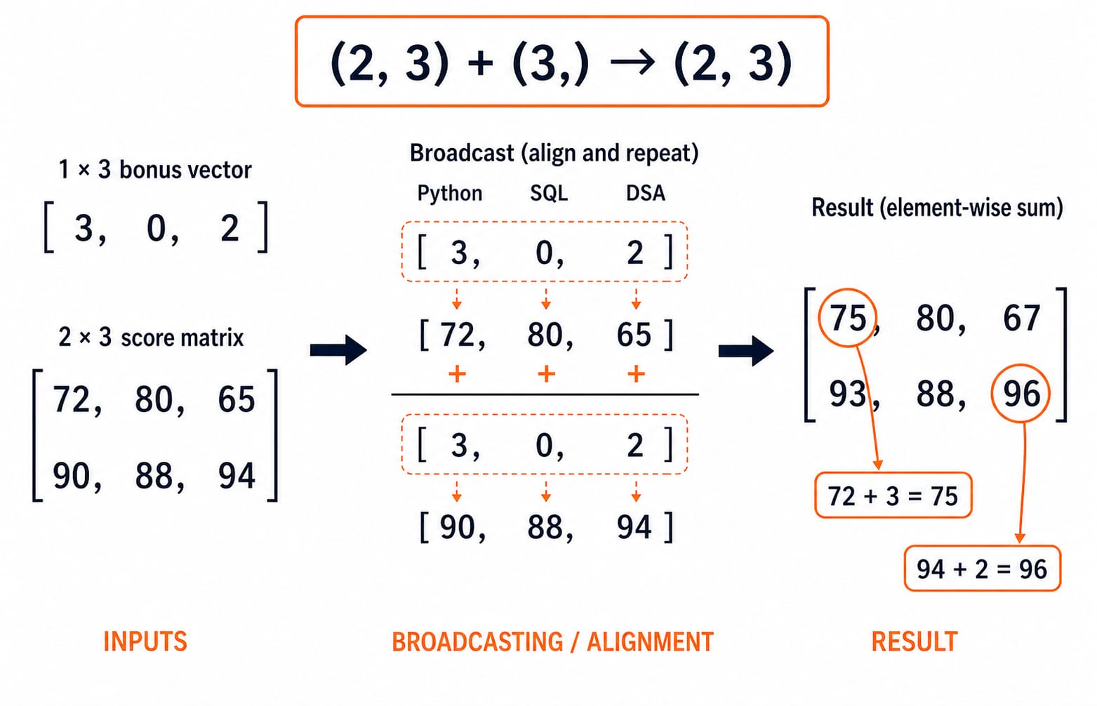
The input shapes are (2, 3) and (3,). Under NumPy's official broadcasting rules, dimensions are compared from the right. The bonus length 3 therefore aligns with the last dimension of marks.

Student A becomes [72 + 3, 80 + 0, 65 + 2] = [75, 80, 67]. Student B becomes [90 + 3, 88 + 0, 94 + 2] = [93, 88, 96]. Thus:

adjusted = [[75, 80, 67],
            [93, 88, 96]]

It is useful to imagine the bonus aligned with both rows, but the code does not manually create a second bonus row. Adding np.array([1, 2]) fails with ValueError: trailing lengths 3 and 2 are neither equal nor 1. Broadcasting is not repetition in every direction.

5. Aggregate, transpose, reshape and sort by axis

adjusted.sum(axis=1) reduces each row and returns shape (2,). The totals are 75 + 80 + 67 = 222 and 93 + 88 + 96 = 277, so the result is [222, 277].

adjusted.mean(axis=0) reduces the student axis and leaves one value per subject, shape (3,). Python gives (75 + 93) / 2 = 84.0, SQL gives (80 + 88) / 2 = 84.0, and DSA gives (67 + 96) / 2 = 81.5. The result is [84.0, 84.0, 81.5].

Transpose and reshape are not interchangeable:

adjusted.T
array([[75, 93], [80, 88], [67, 96]], dtype=int32)

adjusted.reshape(3, 2)
array([[75, 80], [67, 93], [88, 96]], dtype=int32)

Transpose swaps the axes. Reshape preserves element order and changes the grouping. Finally, np.sort(adjusted, axis=1) sorts within each student's row and returns [[67, 75, 80], [88, 93, 96]] without changing adjusted. Sorting Algorithms: Complexity and Comparison explains the broader algorithmic idea, not NumPy's internal sort choice.

6. Understand views, copies and three common traps

Basic slicing often creates a view, as NumPy's official copies and views guide explains:

base = np.array([10, 20, 30, 40])
window = base[1:3]
window[0] = 99

Now window is [99, 30], and base is [10, 99, 30, 40] because the slice shares data. Advanced indexing behaves differently. picked = base[[0, 2]] gives [10, 30]. After picked[0] = -1, picked is [-1, 30], while base stays [10, 99, 30, 40]. Use .copy() when independent mutation is the clearest intent.

Three traps are worth checking explicitly:

1. List + concatenates instead of adding. Convert both inputs to arrays.

2. Incompatible shapes fail broadcasting. Inspect .shape from the trailing axes.

3. if marks: raises ValueError because a multi-element array has no single truth value. Ask the real question with a condition followed by .any() or .all(), such as (marks >= 85).any().

7. Predict exact NumPy outputs

Try these before reading the answers:

• np.arange(2, 11, 2) gives [2, 4, 6, 8, 10], shape (5,).

• np.array([1, 2, 3]) * 3 gives [3, 6, 9], shape (3,).

• adjusted[:, 2] gives the DSA column [67, 96], shape (2,).

Now locate the original mark below 70. marks < 70 is true only at row 0, column 2, so np.argwhere(marks < 70) returns [[0, 2]]. That coordinate means Student A's DSA mark 65. The corrected array contains 70 at the same coordinate, while marks still contains 65.

A strong quiz or interview solution follows the same order: write the input shape, trace the selected axes, predict the output shape, then calculate values. For structured array and problem-solving practice, continue with DSA Using Python.

8. NumPy basics in one checklist and the next step

• Create the array with an intentional dtype.

• Inspect shape, ndim and size.

• Track shape while indexing and masking.

• Align trailing dimensions before broadcasting.

• Name the axis before reducing.

• Distinguish transpose from reshape.

• Check whether an operation returns a view or a copy.

The (2, 3) marks array plus the (3,) bonus produced [[75, 80, 67], [93, 88, 96]], row totals [222, 277], and subject means [84.0, 84.0, 81.5]. Rerun the code with a third student row and predict every changed shape before execution. Then use the Python course for language fundamentals or DSA Using Python for broader problem-solving practice.