Multi-Layer Perceptron and Backpropagation Explained with a Worked Example
Build a 2-2-1 neural network from its inputs to its loss, then trace backpropagation through every weight and bias. The complete update shows why each sign matters.
KnowledgeGate Team
Exam prep & CS education
Updated 26 Aug 20265 min read93 views
Backpropagation becomes confusing when activations, errors, gradients, and updated weights reuse similar symbols. With fixed initial parameters, a 2-2-1 Multi-Layer Perceptron turns one training sample into a prediction, a loss, nine gradients, and one simultaneous parameter update. Carrying every number through the calculation makes the direction and sign of each update easy to check.
Related reading: backpropagation MCQs and neural network forward passes.
Multi-Layer Perceptron structure: what each layer does
A perceptron takes a weighted sum of its inputs, adds a bias, and applies an activation function. A Multi-Layer Perceptron, or MLP, is a feed-forward network with at least one hidden layer. The input layer only holds the feature values. Hidden neurons transform those values, and the output neuron produces the prediction.
Here, z_h denotes a hidden neuron's weighted sum before activation, a_h its activation, z_o the output pre-activation, and y_hat the prediction. In compact form:
h = sigma(W1 x + b1)
y_hat = sigma(W2 h + b2)
Naming every edge makes the matrix orientation unambiguous. Unlike hand-written symbolic rules, an MLP learns by adjusting numerical weights. Artificial Neural Networks: Complete Guide with Worked Examples for GATE and Interviews provides the broader context on neurons, activation functions, perceptron learning, and linear separability. An MLP adds a hidden-layer delta that receives error through the original output weights.
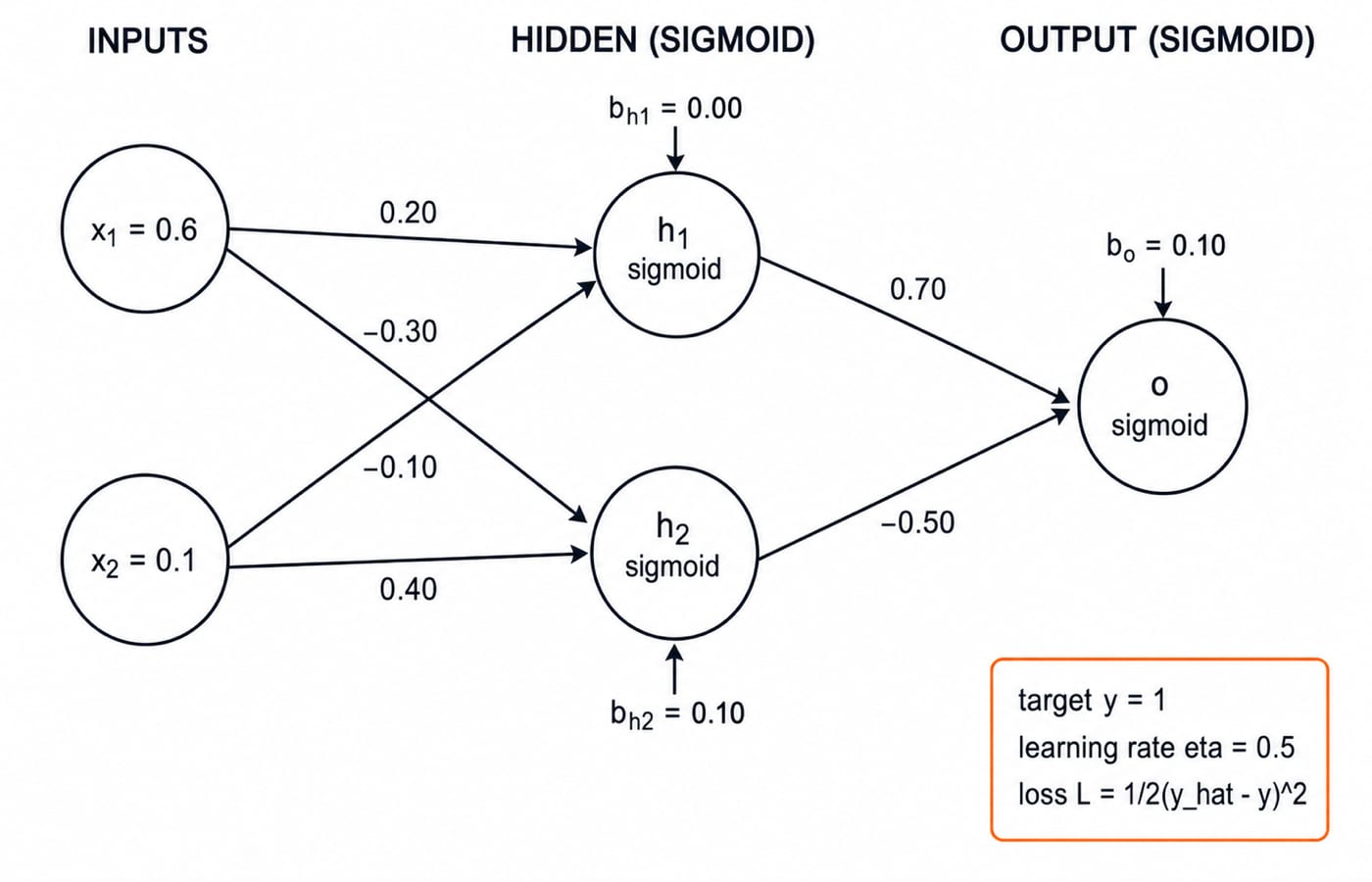
Forward propagation: from features to a prediction
Each neuron repeats three operations: multiply inputs by weights, add the bias, then apply the activation. Here the activation is sigmoid(z) = 1 / (1 + e^(-z)) at both hidden and output neurons.
Non-linearity matters. Without a non-linear activation, several dense layers collapse into one linear transformation. ReLU is a common hidden-layer alternative. Both hidden and output neurons use sigmoid here, so every derivative remains visible. For sigmoid, the useful identity is sigmoid'(z) = sigmoid(z)(1 - sigmoid(z)), or simply a(1 - a). A stored activation can therefore be reused in the backward pass.
Backpropagation: the chain rule in reverse
Backpropagation applies the chain rule efficiently. From the scalar loss, it traces influence backwards through the output activation, output pre-activation, output weights, hidden activations, hidden pre-activations, and input-to-hidden weights.
For squared error and a sigmoid output, the output delta is:
delta_o = (y_hat - y)y_hat(1 - y_hat)
Using the old downstream output weight v_j, each hidden delta is:
delta_hj = delta_o v_j a_hj(1 - a_hj)
The gradients are dL/dv_j = delta_o a_hj, dL/dw_ij = delta_hj x_i, and dL/db = delta. Gradient descent then applies parameter_new = parameter_old - eta * gradient. The minus sign already belongs to the update rule, so do not reverse the error term again.
Worked example, part 1: compute the complete forward pass
Take x1 = 0.6, x2 = 0.1, target y = 1, learning rate eta = 0.5, and L = 1/2(y_hat - y)^2.
For hidden neuron h1:
z_h1 = (0.6)(0.20) + (0.1)(-0.10) + 0.00 = 0.110000
a_h1 = sigmoid(0.11) = 0.527472
For hidden neuron h2:
z_h2 = (0.6)(-0.30) + (0.1)(0.40) + 0.10 = -0.040000
a_h2 = sigmoid(-0.04) = 0.490001
At the output:
z_o = (0.527472)(0.70) + (0.490001)(-0.50) + 0.10 = 0.224230
y_hat = sigmoid(0.224230) = 0.555824
L = 1/2(0.555824 - 1)^2 = 0.098646
Worked example, part 2: backpropagate and update every parameter
Begin at the output:
delta_o = (0.555824 - 1)(0.555824)(1 - 0.555824) = -0.109660
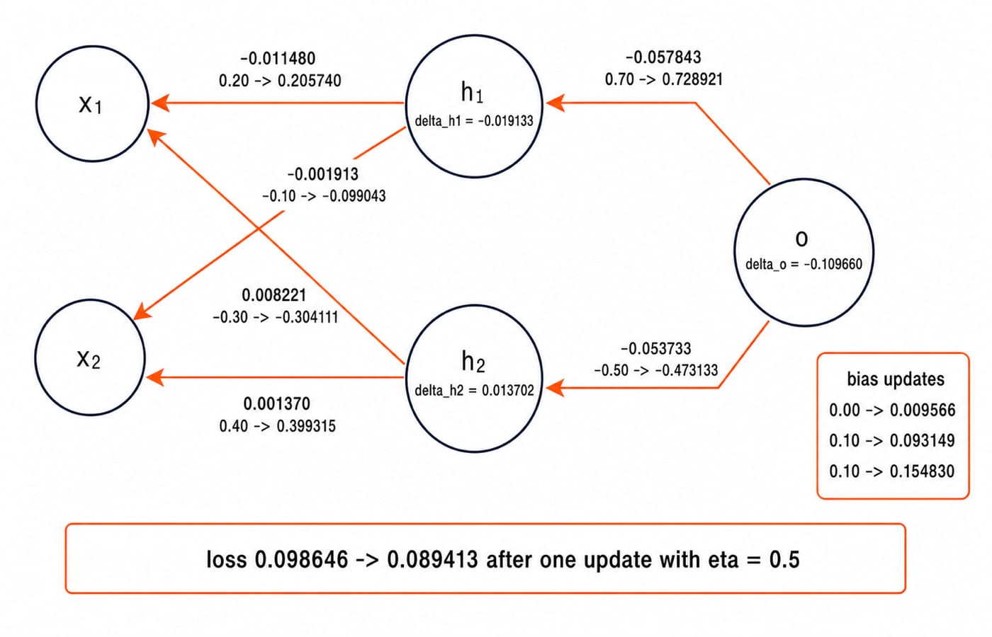
Therefore, dL/dv_h1o = -0.109660(0.527472) = -0.057843, dL/dv_h2o = -0.109660(0.490001) = -0.053733, and dL/db_o = -0.109660.
Now use the original output weights, 0.70 and -0.50, for the hidden deltas:
delta_h1 = -0.109660(0.70)(0.527472)(1 - 0.527472) = -0.019133
delta_h2 = -0.109660(-0.50)(0.490001)(1 - 0.490001) = 0.013702
Multiplying each hidden delta by its input gives dL/dw_x1h1 = -0.011480, dL/dw_x2h1 = -0.001913, dL/dw_x1h2 = 0.008221, and dL/dw_x2h2 = 0.001370. The bias gradients are the deltas themselves: dL/db_h1 = -0.019133 and dL/db_h2 = 0.013702.
Apply theta_new = theta_old - 0.5 * gradient to every parameter only after all gradients are known.
Parameter | Old value | Gradient | New value |
|---|---|---|---|
| 0.200000 | -0.011480 | 0.205740 |
| -0.100000 | -0.001913 | -0.099043 |
| 0.000000 | -0.019133 | 0.009566 |
| -0.300000 | 0.008221 | -0.304111 |
| 0.400000 | 0.001370 | 0.399315 |
| 0.100000 | 0.013702 | 0.093149 |
| 0.700000 | -0.057843 | 0.728921 |
| -0.500000 | -0.053733 | -0.473133 |
| 0.100000 | -0.109660 | 0.154830 |
Running the same sample forward with these updated values gives y_hat_new = 0.577122 and L_new = 0.089413. The loss is lower than 0.098646. One step does not need to solve the example. It only needs to move the chosen loss downhill.
Common backpropagation traps and how to correct them
Keep a four-column scratch table for each neuron: z, activation, delta, and gradient. Carry six decimals until the end, then round the result. This prevents symbols from changing meaning.
All gradients in one training step must come from the same forward-pass parameter snapshot. If you update the output weights before computing hidden deltas, you mix two network states. Calculate every gradient first, then update all parameters together.
Other common errors are dropping the activation derivative, using y - y_hat without changing the update convention, and forgetting that every bias has a gradient. Sigmoid saturation matters too. An activation near 0 or 1 has a small derivative, which can shrink gradients across many layers.
A falling loss on one sample is useful, but it is not complete proof. Check tensor shapes, perform a tiny numerical gradient check, and watch the loss across several examples.
How exams test MLPs and backpropagation
Questions commonly ask you to identify an architecture or activation, count trainable parameters, execute one forward pass or update, or diagnose vanishing gradients, learning-rate behaviour, and sign errors. For example, a fully connected 4 input -> 3 hidden -> 2 output MLP has (4 x 3 + 3) + (3 x 2 + 2) = 15 + 8 = 23 trainable parameters when both layers have biases.
The answer format changes how a calculation should be checked, so review MCQ, MSQ or NAT? GATE Question Types Explained. For broader preparation, the GATE CS Exam page organises subject-wise study paths.
The short version and the next practice step
Forward propagation makes the prediction.
The loss measures the prediction error.
Backpropagation computes local chain-rule deltas from output to input.
Gradient descent updates every parameter opposite its gradient.
In this example, one simultaneous update reduced the loss from 0.098646 to 0.089413. Reproduce the 2-2-1 calculation without looking, then change only x2 from 0.1 to 0.2 and recompute the forward pass before attempting another complete update.
For a wider learning path, continue with Artificial Intelligence (AI). GATE aspirants who want structured subject-wise preparation can use GATE Guidance by Sanchit Sir.
Keep learning

Problem Representation in AI: State Space, Worked Water-Jug Example and Exam Traps
Learn how states, operators, goals and costs turn a verbal task into a search problem. The worked water-jug trace separates valid states from reachable ones.
Updated 23 Oct 20265 min readML & Data Science

Foundations and Evolution of AI: Approaches, Timeline and a Worked Rational-Agent Example
Build a connected map of AI foundations, historical shifts and major paradigms, then calculate how a rational agent chooses under uncertainty.
Updated 19 Oct 20266 min readML & Data Science

Natural Language Processing Explained: Pipeline, TF-IDF Worked Example and Exam Patterns
Start from raw text, build BoW and TF-IDF vectors, compute cosine similarity, examine ambiguity, and finish with evaluation and exam-style checks.
Updated 15 Oct 20266 min readML & Data Science

Fundamentals of Planning in AI: STRIPS, State-Space Search and a Worked Blocks World Plan
Build a planning problem from facts, actions and goals, then follow every add and delete effect through a complete six-step Blocks World solution.
Updated 11 Oct 20266 min readML & Data Science