Hashing and collision resolution: hash functions, chaining and open addressing
Hashing and collision resolution explained: hash functions, load factor, separate chaining, and open addressing with linear, quadratic and double hashing.
KnowledgeGate Team
Exam prep & CS education
Updated 16 Jul 20266 min read
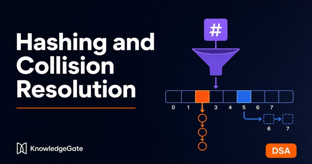
Hashing is how a data structure achieves the near-impossible: average O(1) insert, search, and delete, independent of how many items it holds. The idea is simple. Convert a key into an array index with a hash function, and store the item there. The trouble is that two different keys can map to the same index, a collision, and everything interesting about hashing is how you resolve them. Get the two resolution families straight and tracing a probe table or computing expected probes at a given load factor becomes mechanical.
Hash functions: turning a key into an index
A hash function h maps a key k to an index in the range 0 to m − 1, where m is the table size. A good hash function has two properties: it is fast to compute, and it spreads keys uniformly across the table so collisions are rare. The most common design is the division method, h(k) = k mod m, which is why m is usually chosen as a prime not close to a power of two, to avoid patterns in the low bits clustering keys. The multiplication method multiplies k by a constant fraction and takes the fractional part, and is less sensitive to the choice of m.
The one number that governs performance is the load factor, defined as α = n / m, the ratio of stored items n to table slots m. As α rises, collisions rise, and every resolution scheme degrades. Keeping α bounded, typically below 0.7 for open addressing, is what preserves the O(1) promise. When α gets too high the table is rehashed into a larger array.
Separate chaining: a list per slot
In separate chaining each table slot holds a linked list (a chain) of all the keys that hash there. To insert, compute h(k) and append to that slot's list. To search, compute h(k) and scan only that one short list.
The table never fills, so α can exceed 1; a load factor of 2 just means average chains of length 2.
Average search cost is O(1 + α), the constant one for the hash plus the expected chain length. With a good hash and bounded α, that is O(1).
The cost is the pointer overhead of the lists and poor cache behaviour, since chained nodes are scattered in memory.
Chaining is the forgiving choice: deletion is trivial, and performance degrades gently as the table fills.
Open addressing: everything in the table
Open addressing stores every key inside the array itself, no external lists. On a collision it probes a deterministic sequence of alternative slots until it finds an empty one. The three probe sequences you must know differ only in how they compute the next slot.
Linear probing: try h(k), then h(k)+1, h(k)+2, and so on, modulo m. Simple and cache-friendly, but it suffers primary clustering, where occupied slots merge into long runs that lengthen every future probe.
Quadratic probing: try h(k), then h(k)+1², h(k)+2², h(k)+3², modulo m. This breaks up the long runs of linear probing, trading primary clustering for milder secondary clustering (keys with the same initial slot still follow the same probe path).
Double hashing: use a second hash function for the step size, probing h(k), then h(k)+1·h₂(k), h(k)+2·h₂(k), and so on. Different keys get different step sizes, which all but eliminates clustering and is the highest-quality open-addressing scheme.
Because open addressing has no lists, it lives or dies by the load factor: once α approaches 1 the table is nearly full and probe sequences grow very long. Deletion also needs care, since a naive removal would break the probe chains that pass through the emptied slot, so removed slots are marked with a special deleted tombstone rather than truly cleared.
A worked insert sequence with probing
Take a table of size m = 10 with h(k) = k mod 10, and insert the keys 12, 22, 32, 42, 35 in order using linear probing. The first four keys all hash to index 2, a deliberate pile-up that shows collisions clearly.
Key | h(k) | Probe sequence | Lands at |
|---|---|---|---|
12 | 2 | slot 2 empty | 2 |
22 | 2 | 2 taken, try 3 | 3 |
32 | 2 | 2, 3 taken, try 4 | 4 |
42 | 2 | 2, 3, 4 taken, try 5 | 5 |
35 | 5 | 5 taken, try 6 | 6 |
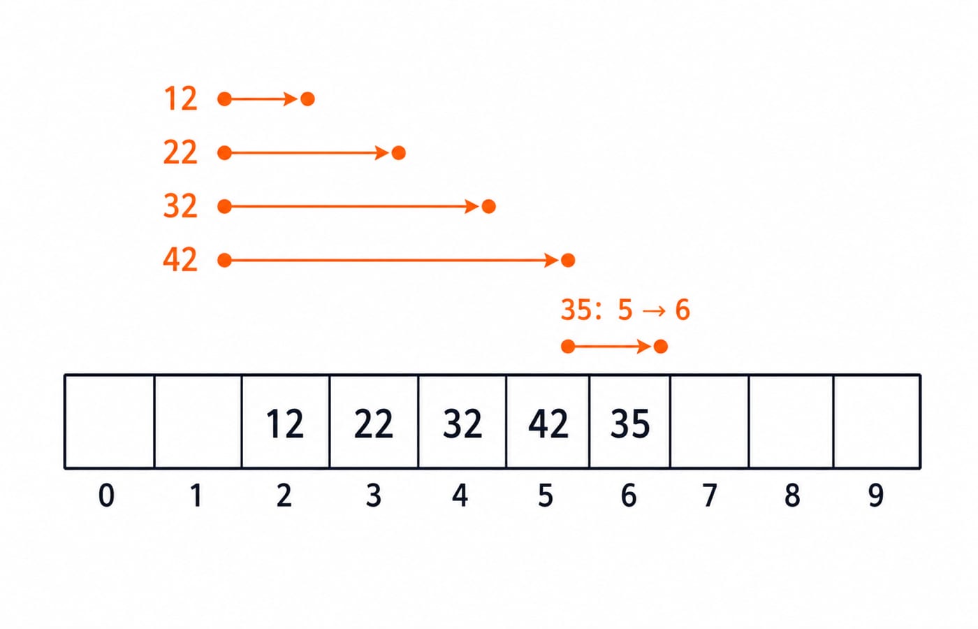
Notice the last insert. Key 35 hashes cleanly to slot 5, but slot 5 is already occupied by 42, which had drifted there from the earlier cluster. This is primary clustering in action: one crowded region makes an unrelated key probe further. Under double hashing with h₂(k) = 7 − (k mod 7), the same four keys step by 2, 6, 3 and 7 and land in slots 2, 8, 5 and 9 instead. They still collide on their home slot, but they no longer merge into a run, so slots 3 and 4 stay free for the keys that genuinely hash there. That is what double hashing buys you: it removes the runs, not the collisions.
Average lookup cost
The point of bounding α is a predictable cost. For separate chaining, a successful search averages about 1 + α/2 comparisons and an unsuccessful one about 1 + α. For open addressing with uniform probing, an unsuccessful search averages about 1 / (1 − α) probes: at α = 0.5 that is 2 probes, but at α = 0.9 it jumps to 10. That non-linear blow-up near a full table is the reason open-addressing tables are rehashed well before they fill, and it is a favourite numerical.
Chaining vs open addressing: choosing between them
The two families fail in different directions, and that is what decides between them. Separate chaining is the safer default when the key count is not bounded in advance, or when deletions are frequent: a heavily loaded table costs you slow lookups, never a broken probe chain. Open addressing wins on memory locality, everything in one contiguous array with no pointers to chase, but it obliges you to rehash before α climbs near 1.
Separate chaining | Open addressing | |
|---|---|---|
Where a key lives | In a linked list hanging off its slot | In the table array itself |
Load factor α | May exceed 1; chains simply get longer | Must stay below 1, and in practice under about 0.7 |
Unsuccessful search | About 1 + α comparisons | About 1 / (1 − α) probes |
Deletion | Unlink the node from its chain | Leave a tombstone, or later probes stop early |
Memory and cache | One pointer per node, nodes scattered | No pointers, contiguous and cache-friendly |
How hashing is tested
GATE CS asks you to trace exactly the kind of insert sequence above: given a hash function and a probe method, show the final table or find which slot a key lands in. It asks for the load factor, the expected probes for a successful or unsuccessful search at a given α, and the difference between primary and secondary clustering. Conceptual questions contrast chaining with open addressing and ask which handles a high load factor better (chaining). KnowledgeGate's question bank carries over 130 questions on hashing, and the companion set Hashing MCQs: 12 solved questions works through a representative selection with full explanations.
Placement interviews treat the hash table as the default structure for "find duplicates", "two-sum", and "first non-repeating character", and often ask you to explain collision handling and why a good hash matters. The reasoning is the same, applied to code, and the CS Fundamentals category is where that interview-facing practice sits.
The short version
A hash function maps keys to slots and should spread them uniformly; the load factor α = n/m decides how well any scheme performs. Separate chaining keeps a list per slot and tolerates a high α gracefully. Open addressing packs everything into the array and probes on collision, using linear, quadratic, or double hashing, each better than the last at avoiding clustering. Trace one linear-probing insert sequence and compute the expected probes at two load factors, and the topic is yours.
Drill the traces and cost numericals, then use the Data Structures learn module as your solved-problem hub.
For a GATE-depth sequence that places hashing alongside the rest of the paper, GATE Guidance by Sanchit Sir is built for it.
Hand-fill one probe table and one load-factor cost, and hashing becomes the reliable O(1) tool it is meant to be.
Keep learning
Array Data Structure: Memory Layout, Operations and Worked Examples
Understand how arrays map indices to memory, then practise address calculation, exact shift counts, searching and dynamic-array growth with worked examples.
Updated 24 Oct 20266 min readDSA & Algorithms
Tree Data Structure: Types, Traversals and a Worked BST Example
Build one nine-node binary search tree, classify its shape, trace four traversals, and work through insertion, search, deletion and complexity checks.
Updated 21 Oct 20266 min readDSA & Algorithms
Graphs in Data Structures: Complete Guide with BFS, DFS and Dijkstra Worked Examples
Learn graph terminology, representations and algorithm selection by tracing one unweighted graph with BFS and DFS, then solving a weighted graph with Dijkstra.
Updated 17 Oct 20266 min readDSA & Algorithms

Physical Security and Cryptography Basics: Controls, Keys and Worked Examples
Learn how physical and cryptographic controls work together, then apply them in a four-asset server-room model and a step-by-step toy RSA example.
Updated 13 Oct 20265 min readDSA & Algorithms