GATE DA Machine Learning Revision Map: From Probability to Neural-Network Calculations

Probability, optimisation, classifiers, clustering and neural networks often survive revision as five disconnected note sets. You remember formulas but cannot see which calculation feeds the next. Four small worked problems address probability, optimisation, classification and clustering, followed by a neural-network forward pass. The archived official GATE 2026 material places machine learning under DA, not CS, so this is for a CS-background learner revising GATE DA machine learning.

1. GATE DA machine learning: set the scope before revising

The archived official GATE 2026 paper-and-syllabus page separates CS from DA. Use the archived DA syllabus to verify the topics and exact scope of your own cycle.

These resources support learning, not the official DA syllabus. The UGC NET Computer Science Machine Learning Revision Map follows Units 4 and 10 through seven sessions; GATE DA instead connects probability, gradient descent, k-NN, k-means and one neural-network inference in a 90-minute loop.

The dependency chain is simple: probability estimates uncertainty; an objective function measures error; optimisation changes parameters; a classifier or clusterer turns parameters or distances into structure; a neural network repeats weighted sums and nonlinear activations.

2. Probability for machine learning: compute a posterior

In a toy binary classifier, let P(C1)=0.6 and P(C0)=0.4. For observed A=1 and B=1, use P(A=1|C1)=0.8, P(B=1|C1)=0.5, P(A=1|C0)=0.3 and P(B=1|C0)=0.9. Naive Bayes assumes conditional independence given the class.

0.6 x 0.8 x 0.5 = 0.240

0.4 x 0.3 x 0.9 = 0.108

P(C1 | A=1, B=1) = 0.240 / (0.240 + 0.108) = 0.690

P(C0 | A=1, B=1) = 0.108 / 0.348 = 0.310

The prediction is C1. Comparing 0.240 with 0.108 chooses the class, but calling 0.240 the posterior is wrong because it is not normalised.

3. Optimisation and logistic regression: make one gradient update

Use one training point x=2, y=1, initial weight w=1, bias b=-1.5 and learning rate 0.1.

z = wx + b = (1 x 2) - 1.5 = 0.5

p = sigmoid(0.5) = 0.622459...

The binary cross-entropy loss is L = -ln(0.622459...) = 0.474. The gradients are:

dL/dw = (p-y)x = (0.622459...-1) x 2 = -0.755

dL/db = p-y = 0.622459...-1 = -0.378

Apply gradient descent:

w_new = 1 - 0.1(-0.755) = 1.0755

b_new = -1.5 - 0.1(-0.378) = -1.4622

Because y=1 but p=0.622, both updates raise the logit. Common errors are subtracting a y-p gradient, dropping x from dL/dw, and rounding p before finding the loss.

4. Classification calculations: let distance produce the decision

Take labelled points A=(0,2), class 0; B=(2,1), class 0; C=(3,3), class 1; D=(4,5), class 1; and query Q=(2,3). Their Euclidean distances from Q are:

For k=3, take C at 1.000, B at 2.000, then A at 2.236. Labels 1, 0 and 0 classify Q as 0 by a 2-to-1 vote. No distance tie affects the neighbour order; a tied class vote would still need a stated rule.

Logistic regression learns a boundary by minimising loss. k-NN stores examples and decides locally by distance. Scale features first, or a large-unit feature can dominate that distance.

5. Clustering calculations: assign, update and measure

Use unlabelled points P1=(1,1), P2=(1,2), P3=(4,4) and P4=(5,4), with initial centroids M1=(1,1) and M2=(5,4).

P1 is 0 from M1 and 5 from M2. For P2, d(P2,M1)=1 versus d(P2,M2)=sqrt(20). For P3, d(P3,M1)=sqrt(18) versus d(P3,M2)=1. P4 is 5 from M1 and 0 from M2. Thus P1 and P2 join cluster 1; P3 and P4 join cluster 2.

Update each centroid using its assigned points:

M1' = ((1+1)/2, (1+2)/2) = (1,1.5)

M2' = ((4+5)/2, (4+4)/2) = (4.5,4)

The within-cluster sum of squared errors is 0.25 + 0.25 + 0.25 + 0.25 = 1.00.

Classification uses known labels; clustering discovers groups without them. Traps include updating a centroid before all assignments, mixing distance with squared distance in the objective, and expecting every initialisation to agree.

6. Neural-network calculations: trace a two-layer forward pass

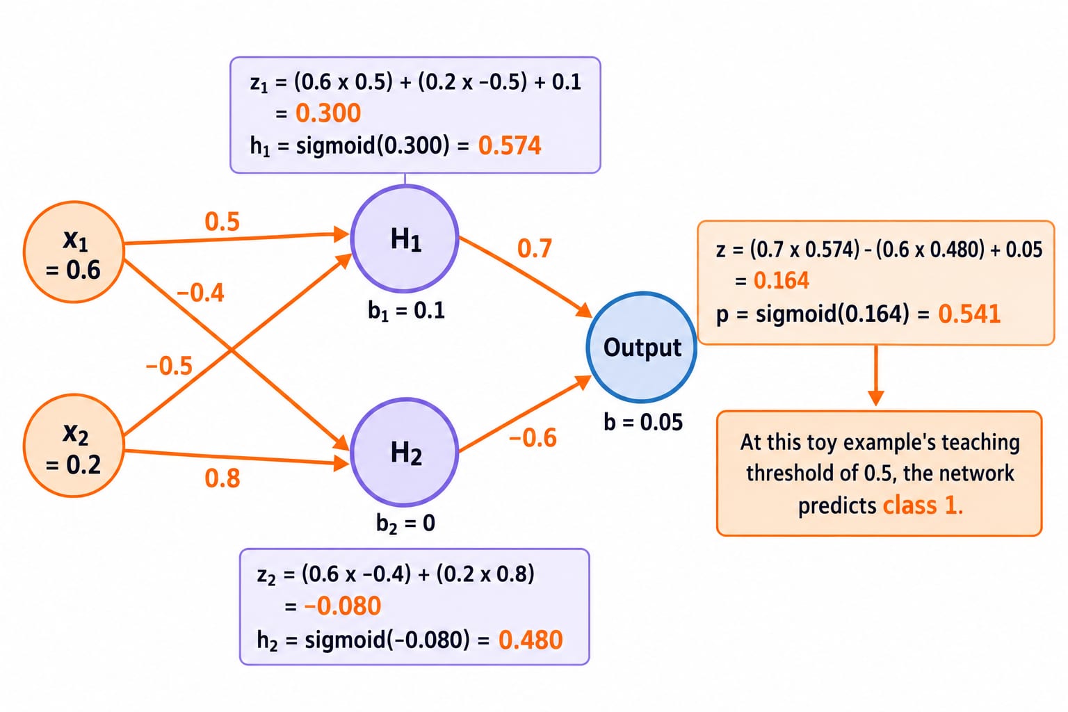
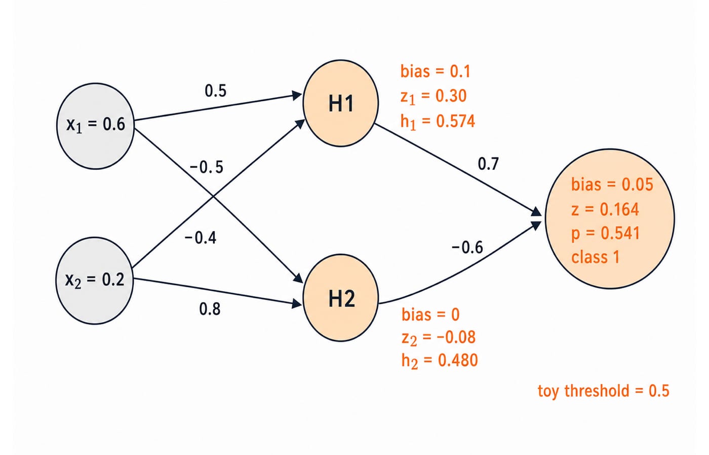
Let x1=0.6 and x2=0.2. Hidden neuron H1 has weights 0.5 and -0.5 with bias 0.1:

z1 = (0.6 x 0.5) + (0.2 x -0.5) + 0.1 = 0.300

h1 = sigmoid(0.300) = 0.574

Hidden neuron H2 has weights -0.4 and 0.8 with bias 0:

z2 = (0.6 x -0.4) + (0.2 x 0.8) = -0.080

h2 = sigmoid(-0.080) = 0.480

The output neuron uses weights 0.7 from H1 and -0.6 from H2, with bias 0.05:

z = (0.7 x 0.574) - (0.6 x 0.480) + 0.05 = 0.164

p = sigmoid(0.164) = 0.541

At this toy example's teaching threshold of 0.5, the network predicts class 1. This is not an official exam rule.

7. GATE DA machine learning revision: a 90-minute loop

1. Take 15 minutes to recompute and normalise the Bayes scores.

2. Take 20 minutes to redo the logistic loss and gradient update.

3. Take 15 minutes to rank the four k-NN distances.

4. Take 15 minutes for the k-means assignment, centroid update and SSE.

5. Take 15 minutes to trace the neural-network forward pass.

6. Take 10 minutes to record one error per block.

The total is 15 + 20 + 15 + 15 + 15 + 10 = 90 minutes. Keep a five-column error sheet: concept, wrong step, corrected calculation, reason, and one fresh value change.

For a transfer test, change the logistic point to x=1 while retaining y=1, w=1 and b=-1.5. Obtain z = (1 x 1) - 1.5 = -0.5 and p = sigmoid(-0.5) = 0.378 before finding the new gradient.

The short version

Revise in dependency order and require a numerical output each time. Use Engineering Mathematics for probability, calculus and linear algebra. Use the GATE CS category for broader CS preparation. Neither is a DA-specific complete course.