Silhouette Score vs Inertia: Compare Clustering Quality with a Worked Example

Inertia and silhouette can rank the same partitions differently, so “lower is better” and “higher is better” do not settle which one to trust. The ordered dataset is X = {0, 1, 2, 3, 8, 9, 10, 11}. Clustering A forms two natural groups; Clustering B splits the left group into two. The earlier Unsupervised Learning and Clustering Explained: K-Means Worked Example and Exam Traps establishes representation, distance and k-means updates. The fixed partitions isolate how inertia judges compactness while silhouette balances cohesion against separation.

1. Start with the question each clustering score answers

Inertia is the sum of squared distances from every point to the centroid of its assigned cluster:

J = sum over clusters C of sum over x in C of ||x - mu_C||^2

It asks a local question: how tightly do assigned points sit around their centroids? Lower is better only when the dataset, features, scaling, and distance convention stay fixed.

For point i, silhouette starts with a(i), the mean distance to other points in its own cluster, and b(i), the smallest mean distance to any other cluster:

s(i) = (b(i) - a(i)) / max(a(i), b(i))

The overall score is the mean of all point values. A value near 1 indicates clear separation, one near 0 indicates a boundary point, and a negative value means another cluster is closer on average.

The contrast is simple: inertia measures centroid compactness, and its best achievable value cannot increase as more clusters are allowed. Silhouette compares cohesion with separation and can fall after a natural group is split. Neither score is accuracy because no class labels exist here.

2. Calculate inertia for the natural two-cluster partition

Fix Clustering A as A1 = {0, 1, 2, 3} and A2 = {8, 9, 10, 11}. Their centroids are:

mu_A1 = (0 + 1 + 2 + 3) / 4 = 1.5

mu_A2 = (8 + 9 + 10 + 11) / 4 = 9.5

For A1, show every squared distance:

(0 - 1.5)^2 + (1 - 1.5)^2 + (2 - 1.5)^2 + (3 - 1.5)^2

= 2.25 + 0.25 + 0.25 + 2.25 = 5

The second cluster is symmetric, so it also contributes 5. Therefore inertia(A) = 5 + 5 = 10.

This establishes compactness relative to a one-cluster fit, but 10 has no universal good-or-bad meaning. Double every coordinate to {0, 2, 4, 6, 16, 18, 20, 22} and the centroids become 3 and 19. Every distance doubles, every squared distance becomes four times larger, and the same partition has inertia 40. Inertia values from different scales are not directly comparable.

3. Calculate the silhouette score point by point

For x = 3 in A, the within-cluster distances to {0, 1, 2} are 3, 2, 1. Thus:

a(3) = (3 + 2 + 1) / 3 = 2

Its distances to {8, 9, 10, 11} are 5, 6, 7, 8, so:

b(3) = (5 + 6 + 7 + 8) / 4 = 6.5

s(3) = (6.5 - 2) / 6.5 = 4.5 / 6.5 = 0.692

Check a less exposed point, x = 1. Here a(1) = (1 + 1 + 2) / 3 = 4/3 and b(1) = (7 + 8 + 9 + 10) / 4 = 8.5. Therefore s(1) = (8.5 - 4/3) / 8.5 = 0.843.

The point-level silhouette values in A are:

Average the unrounded values, not the displayed three-decimal values. The result is silhouette(A) = 0.786785..., reported as 0.787.

4. Compare the over-split three-cluster partition

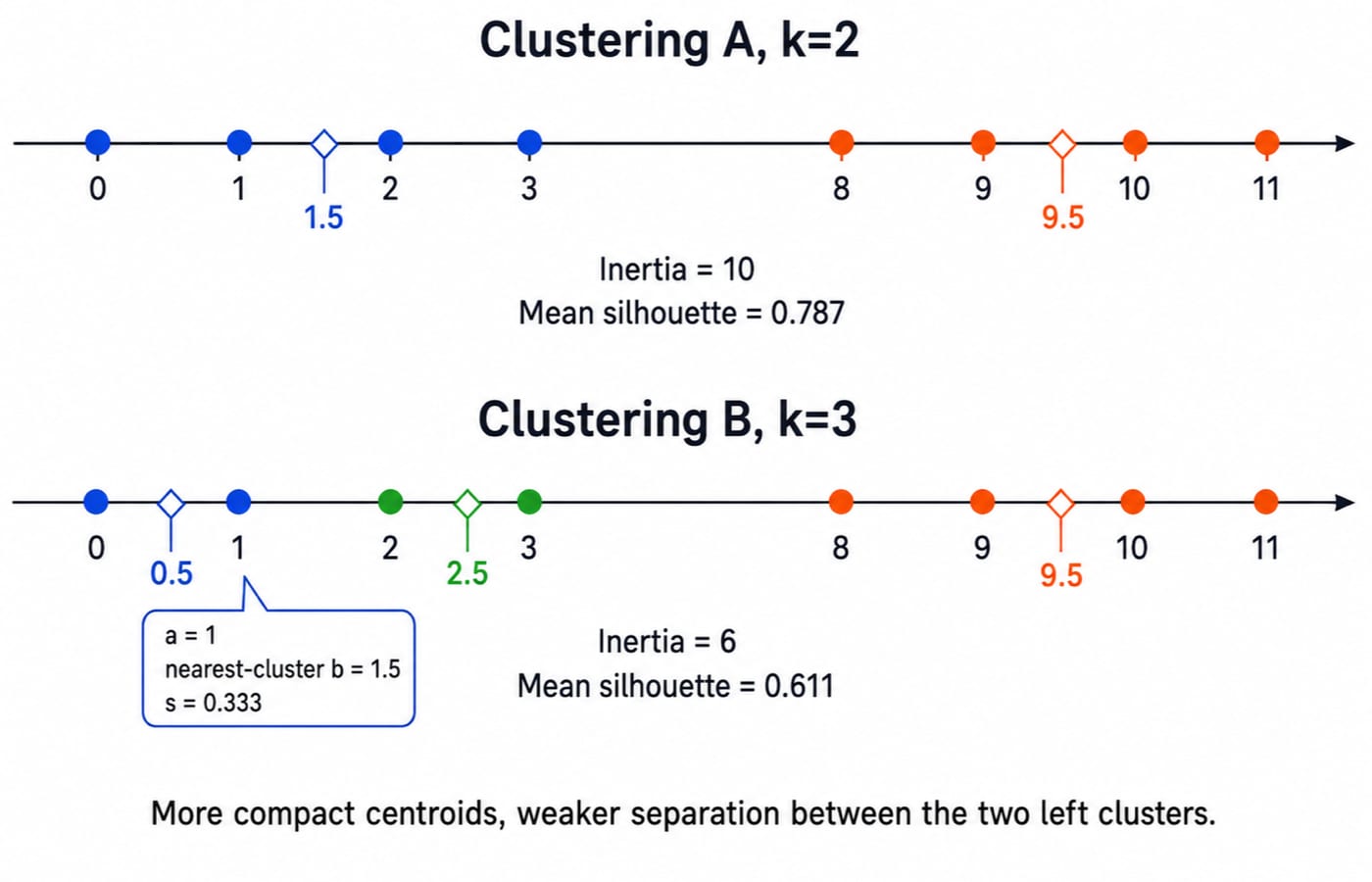
Now fix Clustering B as B1 = {0, 1}, B2 = {2, 3}, and B3 = {8, 9, 10, 11}. Its centroids are 0.5, 2.5, and 9.5. Its inertia is:

[(0 - 0.5)^2 + (1 - 0.5)^2] + [(2 - 2.5)^2 + (3 - 2.5)^2] + 5

= 0.5 + 0.5 + 5 = 6

For the boundary point x = 1, a(1) = 1. Its mean distance to B2 is (1 + 2) / 2 = 1.5, while its mean distance to B3 is (7 + 8 + 9 + 10) / 4 = 8.5. The nearest alternative is therefore B2, so b(1) = 1.5 and s(1) = (1.5 - 1) / 1.5 = 0.333. The point is compact within its pair but poorly separated from the adjacent pair.

The unrounded average is silhouette(B) = 0.610604..., reported as 0.611. Inertia prefers B because 6 < 10, but silhouette prefers A because 0.787 > 0.611. If the two left pairs have no domain meaning, A is more defensible. If they are stable, useful segments supported outside these scores, B still deserves investigation.

5. Understand why adding clusters lowers inertia but may hurt silhouette

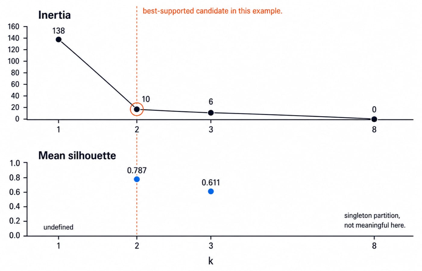
Extend the same dataset across several values of k. With k = 1, the centroid is 5.5 and inertia is 138. Natural A at k = 2 gives 10; B at k = 3 gives 6; one cluster per point at k = 8 gives 0. This is monotonic because an old partition remains available when another centroid is added, so the best achievable inertia cannot get worse.

Silhouette behaves differently. A scores 0.787, while B falls to 0.611 because points 1 and 2 are now close to a neighbouring cluster. Silhouette is undefined for one cluster, and a one-point-per-cluster solution offers no meaningful within-cluster cohesion. Neither extreme is a useful shortcut.

The inertia drop from 138 to 10 is far larger than the drop from 10 to 6, creating an elbow at k = 2 in this example. Silhouette also favours k = 2. Together they support testing A first, but they do not prove that every dataset has a sharp elbow or that any fixed threshold guarantees quality.

6. Avoid comparison traps that change the answer

• Scale trap: Comparing A's inertia 10 with the doubled-coordinate result 40 falsely suggests worse clustering. Fit and compare candidates after one consistent preprocessing pipeline.

• Dataset trap: Inertia from different sample sizes or feature sets is not a same-scale contest. Evaluate candidates on the same data.

• Distance trap: Inertia uses squared distances from centroids, while silhouette can use a chosen distance measure. State the measure and keep the geometry consistent. Uniformly doubling this one-dimensional dataset leaves silhouette unchanged because both a and b double. Changing relative feature scales in multiple dimensions can change neighbours and the score.

• Shape and semantics trap: High silhouette may favour separated, roughly compact groups yet miss non-convex structure, density variation, outliers, unstable assignments, or useless business segments.

Pair both scores with cluster sizes, plots, repeated initialisations or resamples, and domain checks. No threshold such as 0.5 or 0.7 guarantees good clustering.

7. Turn the formulas into an exam check and practical workflow

Useful checkable question forms include:

1. Calculate A's centroids 1.5 and 9.5, then its inertia 10.

2. For point 3, calculate a = 2, b = 6.5, and silhouette 0.692.

3. Explain why inertia selects B while silhouette selects A.

4. Explain why k = 8 reaching inertia 0 is not useful validation.

For a practical run, apply one justified scaling pipeline, fit a small candidate range of k, and record inertia, mean silhouette, and cluster sizes. Inspect point-level silhouettes and outliers, rerun with different seeds or resamples, then decide whether the segments are stable and meaningful.

The short version and next step

Inertia asks how compact clusters are around centroids and tends to reward more clusters. Silhouette asks whether each point is closer to its own cluster than to the nearest alternative. For this dataset, start with A because the elbow and silhouette agree at k = 2, then confirm that choice through stability and domain meaning.

Use the Artificial Intelligence course for the broader AI and machine-learning path and the Python course for implementation foundations. For adjacent practical programmes, browse Skill Development Courses.