Gaussian Mixture Models: Build Soft Clusters with EM Step by Step

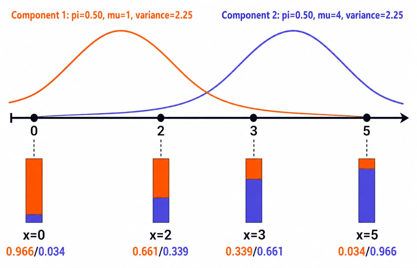
You can see two groups in a data set, but forcing every point into exactly one group feels dishonest. A hard label says, "point 2 belongs to cluster 1", while a soft answer says, "point 2 has 0.661 responsibility for component 1 and 0.339 for component 2". A complete expectation-maximisation cycle produces these probabilities.

Gaussian mixture models turn clusters into probabilities

A Gaussian mixture model (GMM) represents a distribution as a weighted sum of Gaussian components:

p(x) = sum_k pi_k N(x | mu_k, sigma_k^2)

The mixing weights satisfy pi_k >= 0 and sum_k pi_k = 1. Each component has its own centre mu_k and spread sigma_k^2, while pi_k describes the component's share of the population.

For observation x_n, introduce a hidden indicator z_n for the component that generated it. Because that indicator is not observed, the model calculates a responsibility:

gamma_nk = P(z_n = k | x_n)

The responsibilities across all components sum to 1 for each observation. This is the central difference from k-means, which returns one hard cluster label. As a thought check, suppose two equally weighted components have the same density at a point. Their unnormalised scores are equal, so their responsibilities are 0.5 and 0.5. This is conditional membership under the model's current parameters, not a permanent truth about the point.

The earlier Unsupervised Learning and Clustering Explained: K-Means Worked Example and Exam Traps owns feature representation, distance choices, and hard-clustering comparisons. This calculation instead derives probabilistic responsibilities and one complete GMM E-step and M-step.

Set up one two-component model before running EM

Use four one-dimensional observations:

x = {0, 2, 3, 5}

Start with two components and these parameters:

The one-dimensional Gaussian density is:

N(x | mu, sigma^2) = [1 / sqrt(2 pi sigma^2)] exp[-(x - mu)^2 / (2 sigma^2)]

Keep variance 2.25 separate from standard deviation 1.5. Substituting one where the formula expects the other changes every density and responsibility.

In a multivariate GMM, each scalar variance becomes a covariance matrix. Linear Algebra for GATE CS: Eigenvalues and Rank is an optional prerequisite for that extension. Every calculation below stays one-dimensional.

E-step: calculate every soft assignment

The expectation step calculates the probability of each component for each observation:

gamma_nk = pi_k N(x_n | mu_k, sigma_k^2) / sum_j pi_j N(x_n | mu_j, sigma_j^2)

Work through x = 2 first. The two Gaussian densities are:

• N(2 | 1, 2.25) = 0.212965

• N(2 | 4, 2.25) = 0.109340

Multiply by the equal mixing weights:

• Component 1: 0.5(0.212965) = 0.106483

• Component 2: 0.5(0.109340) = 0.054670

Their sum is 0.161153. Normalising each score gives:

• gamma_21 = 0.106483 / 0.161153 = 0.660756

• gamma_22 = 0.054670 / 0.161153 = 0.339244

Repeating the calculation for every observation produces the full responsibility table:

The outer points, 0 and 5, are nearly unambiguous. Points 2 and 3 retain meaningful membership in both components. EM keeps these fractional assignments instead of turning them into hard labels.

M-step: update weights, means, and variances

The maximisation step treats responsibilities as fractional counts. First calculate the effective size of each component:

N_1 = 0.965555 + 0.660756 + 0.339244 + 0.034445 = 2.000000

N_2 = 0.034445 + 0.339244 + 0.660756 + 0.965555 = 2.000000

With n = 4, the weight update is pi_k' = N_k / n. Therefore, pi_1' = pi_2' = 2 / 4 = 0.5.

Next, update component 1's mean with a responsibility-weighted average:

mu_1' ≈ [0(0.965555) + 2(0.660756) + 3(0.339244) + 5(0.034445)] / 2

The approximation sign is needed because the displayed responsibilities are rounded. Using the unrounded values gives a numerator of 2.511469609, so mu_1' = 2.511469609 / 2 = 1.255734805, which rounds to 1.255735.

By symmetry, mu_2' = 3.744265.

The variance update must use the new mean:

sigma_k'^2 = sum_n gamma_nk (x_n - mu_k')^2 / N_k

For component 1, the weighted squared-distance numerator is 3.403608. Dividing by N_1 = 2 gives sigma_1'^2 = 1.701804. Symmetry gives the same result for component 2.

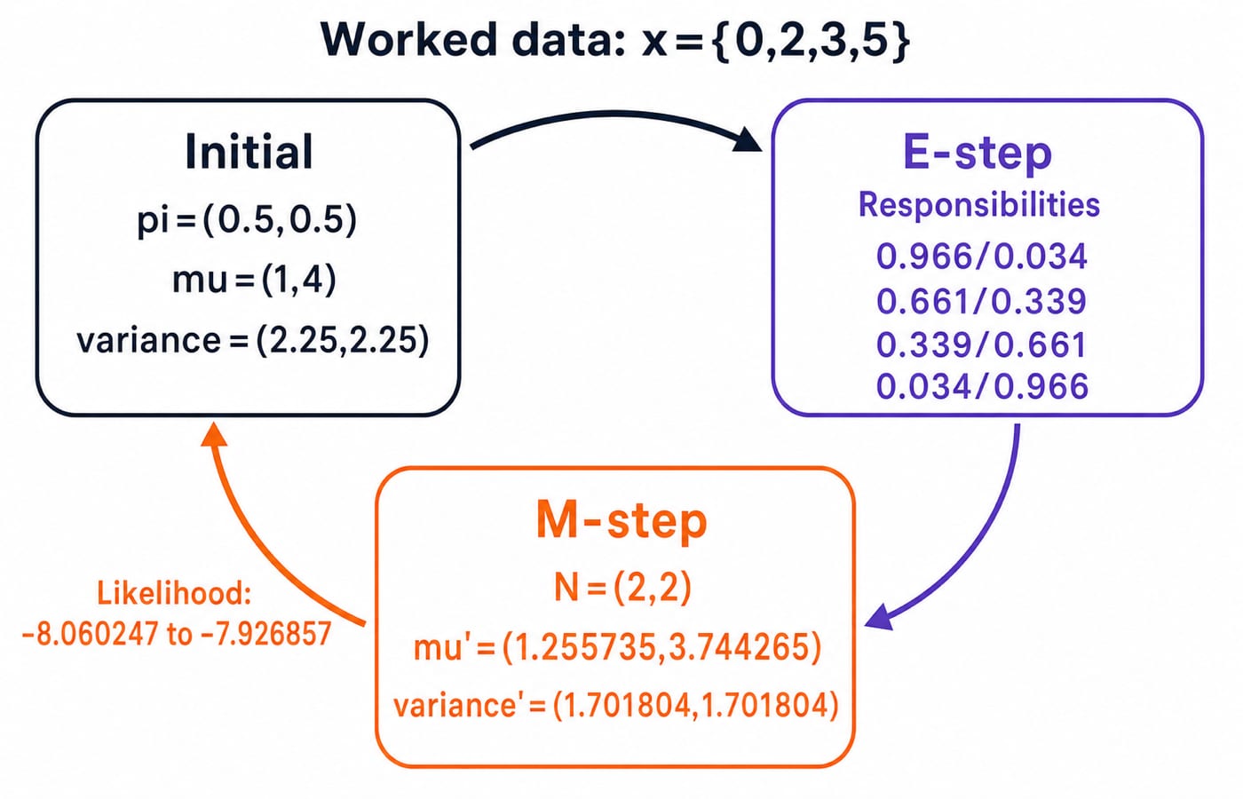
One complete EM cycle has therefore produced:

• (pi_1', mu_1', sigma_1'^2) = (0.5, 1.255735, 1.701804)

• (pi_2', mu_2', sigma_2'^2) = (0.5, 3.744265, 1.701804)

Repeat EM until the likelihood settles

The observed-data log-likelihood measures how well the mixture explains all observations:

L = sum_n log[sum_k pi_k N(x_n | mu_k, sigma_k^2)]

Using the initial parameters gives L = -8.060247. Substituting the updated weights, means, and variances gives L = -7.926857. The second value is less negative, so it is higher and the iteration improved the fit.

The complete loop is precise: initialise the parameters, run the E-step, run the M-step, recompute the log-likelihood, and repeat. Stop when the likelihood improvement is smaller than a chosen tolerance or when a chosen maximum iteration count is reached. Those are implementation choices, not universal constants.

For one-dimensional data, each iteration costs O(nK) for n observations and K components. Time Complexity and Asymptotic Notation explains how to read that expression. EM converges to a stationary solution, but different initial parameters can lead to different local optima.

Common traps that make a GMM answer look plausible but wrong

Formula errors often survive a quick glance. Do not omit pi_k in the E-step, normalise down a component column, put standard deviation where variance belongs, or calculate the new variance around the old mean. Responsibilities must be normalised across components for one observation, and variance must use mu_k'.

Modelling mistakes are equally important. Do not harden responsibilities before the EM update, assume component labels have intrinsic meaning, choose K only because one plot looks convenient, or read a high responsibility as causal certainty.

Real implementations add numerical risks. Tiny densities can underflow, a component can collapse towards zero variance, poor initial values can produce a weak local optimum, and a loose stopping test can halt too early. Use log-space calculations, a small positive variance floor, multiple initialisations, and a plotted likelihood trace as practical checks. No single floor or tolerance is mandatory for every data set.

How concept checks usually test EM and soft clustering

Concept checks ask you to compute a responsibility, perform an M-step, or distinguish GMM from k-means:

1. Compute one responsibility from given weights, means, and variances.

2. Perform one M-step from a responsibility table.

3. Distinguish GMM from k-means by output and geometry. A GMM returns probabilities and can model different component spreads, while k-means returns hard labels based on distances to centroids.

Try two quick checks from our example. What is component 1's responsibility at x = 2? It is 0.660756, or about 0.661. Why do the new mixing weights remain equal? Both effective counts are 2 out of 4 observations.

One diagnostic matters in code: what if a component receives almost no total responsibility? Its N_k becomes tiny, so its mean and variance updates become unstable. This is why component monitoring and variance protection matter.

The short version and the next step

The full chain has five moves. A mixture supplies weighted component densities. The E-step normalises them row by row into responsibilities. The M-step uses those values as fractional counts. The log-likelihood checks progress. Repetition produces soft clusters.

Reproduce the four responsibility rows and both updated means by hand. Then code this single iteration and confirm that the likelihood moves from -8.060247 to -7.926857 before calling a library implementation.

For a wider path through beginner-to-advanced AI and machine learning concepts, continue with Artificial Intelligence (AI): Learn AI and Get Placed. The Skill Development Courses catalogue covers adjacent technical subjects.