Neural Network Architectures: Layers, Forward Passes and Worked Examples

You may recognise the circles and arrows in a neural-network figure but still wonder which layer owns a weight, how many trainable parameters the picture contains, or what value reaches the output. Read any basic architecture through four decisions: what enters, how units connect, where non-linearity is applied, and whether parameters are reused. Dense-network forward passes and connection-pattern examples turn architecture diagrams into calculations.

For the neuron-to-forward-pass foundation, Artificial Neural Networks Explained: Forward Pass, Worked Example and Exam Question Patterns follows one dense network through activation, loss and training. Dense, convolutional and recurrent architectures instead differ in connectivity and in how parameter sharing changes both diagrams and calculations.

What a neural network architecture specifies

An architecture specifies the arrangement of layers, connections, parameter sharing and information flow.

A neuron computes z = sum(w_i x_i) + b, then a = phi(z). Weights and biases are trainable; inputs, pre-activations and activations are temporary. Arrows carry weighted values, and each dense destination unit here has one scalar bias.

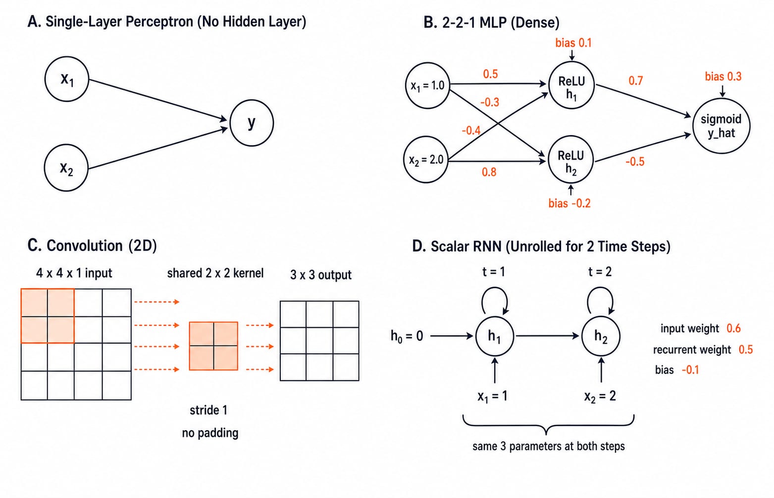
The input layer holds features without weighted computation. A hidden layer sits between input and output, and the output layer produces the prediction. Our 2-2-1 network has two inputs, two hidden ReLU units and one sigmoid output. That means one hidden layer and two trainable layers.

An all-linear stack collapses into one linear transformation. Non-linear ReLU or sigmoid activations can represent boundaries one linear unit cannot.

Main architecture families and their diagram clues

A single-layer feed-forward network connects input directly to output. An MLP adds dense, non-linear hidden layers.

Perceptron and Activation Functions Explained: Worked Examples and Exam Traps calculates a single-neuron update, compares five activations and explains the XOR boundary. MLP, CNN, RNN and encoder-decoder architectures require a different question: which connection pattern the diagram represents.

A CNN applies one small kernel across positions, giving local connections and shared weights. An RNN carries hidden state and reuses one transition across positions. Unrolled copies repeat computation, not parameter sets.

An encoder compresses input into a representation; a decoder expands it. An autoencoder combines both to reconstruct input.

Browse the Coding & Skills category for a broader route through related ideas.

Translate a dense network into equations and parameters

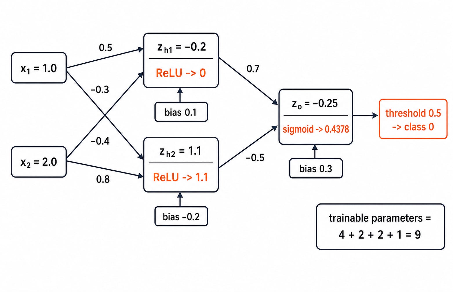
Use column input x = [1.0, 2.0]^T with:

W_h = [[0.5, -0.4], [-0.3, 0.8]], b_h = [0.1, -0.2]^T

W_o = [0.7, -0.5], b_o = 0.3

Calculate z_h = W_h x + b_h, h = ReLU(z_h), z_o = W_o h + b_o, then y_hat = sigmoid(z_o).

The dense-layer rule is n_in x n_out + n_out. A 5-3-2 network has (5 x 3 + 3) + (3 x 2 + 2) = 18 + 8 = 26. A 5-3-4-2 network has 18 + (3 x 4 + 4) + (4 x 2 + 2) = 18 + 16 + 10 = 44, not 26 plus four.

For a full gradient trace and simultaneous nine-parameter update, Multi-Layer Perceptron and Backpropagation Explained with a Worked Example traces gradients and updates all nine parameters. Before gradients, the 2-2-1 forward pass supplies the dense baseline needed to compare CNN and RNN parameter sharing.

Worked forward pass through the 2-2-1 MLP

Compute each weighted sum before its activation.

At an explicitly chosen 0.5 threshold, the class is 0. Keep probability 0.4378 separate from that decision.

Dimensions check: (2 x 2)(2 x 1) + (2 x 1) gives two hidden values; (1 x 2)(2 x 1) + scalar gives one output. Raw z_h1 = -0.2 cannot go onward because ReLU makes it zero.

What parameter sharing changes in CNNs and RNNs

For the CNN, take X = [[1,2,0,1], [0,1,3,2], [2,2,1,0], [1,0,2,1]] with K = [[1,0], [0,-1]], bias 0, stride 1 and no padding. The output side is (4 - 2) / 1 + 1 = 3.

Each 2 x 2 patch contributes its top-left value minus its bottom-right value. The first patch row gives [1 - 1, 2 - 3, 0 - 2] = [0,-1,-2], the second gives [0 - 2, 1 - 1, 3 - 0] = [-2,0,3], and the third gives [2 - 0, 2 - 2, 1 - 1] = [2,0,0]. ReLU therefore gives [[0,0,0], [0,0,3], [2,0,0]].

X = [[1,2,0,1], [0,1,3,2], [2,2,1,0], [1,0,2,1]]

with K = [[1,0], [0,-1]], bias 0, stride 1 and no padding. The output side is (4 - 2) / 1 + 1 = 3. Cross-correlation gives [[0,-1,-2], [-2,0,3], [2,0,0]]; ReLU gives [[0,0,0], [0,0,3], [2,0,0]].

The 2 x 2 x 1 kernel plus bias has 4 + 1 = 5 parameters across nine positions. A dense 16-to-9 map has 16 x 9 + 9 = 153. This compares two toy layers, not universal performance.

For h_t = tanh(0.6x_t + 0.5h_(t-1) - 0.1), use h0 = 0, x1 = 1, x2 = 2. Then h1 = tanh(0.5) = 0.4621, and h2 = tanh(1.2 + 0.5(0.4621) - 0.1) = tanh(1.3311) = 0.8695. The same input weight, recurrent weight and bias serve both steps.

Common architecture traps and repairs

• Counting input circles or forgetting biases: count arrows and destination biases. The main network has nine parameters under either matrix orientation if the convention stays consistent.

• Applying activation too early or too late: finish the weighted sum and bias, apply the activation, then pass that activation onward. Here, z_h1 = -0.2 must become h1 = 0.

• Treating copies as new parameters: nine CNN positions reuse five, and two RNN steps reuse three. Choose from connectivity, sharing and input structure.

How architecture questions test understanding

Architecture questions ask you to identify a network from its connections, count dense or shared parameters, calculate an output shape, trace a forward pass, reject an invalid matrix multiplication, or locate reused weights.

Use these retrieval checks:

1. Main 2-2-1 parameter count? 9.

2. For x = [1,2]^T, what are h1, h2 and y_hat? 0, 1.1 and 0.4378.

3. CNN output shape and parameter count? 3 x 3 and 5.

4. Two-step scalar RNN parameter count? 3, not 6.

Use the retrieval checks as a diagnostic. A missed item points to architecture recognition, parameter counting or forward-pass arithmetic that needs another trace.

The short version and the next step

1. Read the layer sizes.

2. Identify dense, local or recurrent connections.

3. Mark where parameters are shared.

4. Write the affine sum before the activation.

5. Count weights plus destination biases.

Remember dense parameters = n_in x n_out + n_out and convolution output size = floor((N - K + 2P) / S) + 1 for one spatial dimension.

Redraw the 2-2-1 network, hide the solution, recover nine parameters and recompute 0.4378. Then explain the CNN's five shared parameters and the RNN's three. Continue with Artificial Intelligence (AI) for broader study.