Graph Algorithms: BFS, DFS, and shortest paths worked out
Graph algorithms explained: adjacency matrix vs list, BFS and DFS traversal order, edge classification, topological sort, and Dijkstra shortest paths.
KnowledgeGate Team
Exam prep & CS education
Updated 26 Jul 20265 min read
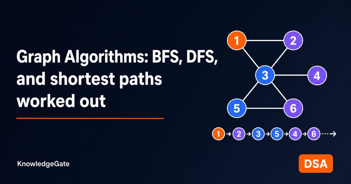
Graphs are where data structures and algorithms meet, and the exam questions on them are mechanical: write down a traversal order, classify a DFS edge, carry out one relaxation step of Dijkstra. Aspirants who can hand-trace those three answer in seconds. Those who half-remember the definitions lose marks on traversal order alone. Everything starts with how the graph is stored.
Graph representations: adjacency matrix vs adjacency list
A graph with V vertices and E edges can be stored two ways.
Adjacency matrix: a V by V grid where entry [u][v] is 1 (or the edge weight) if an edge exists. Space is O(V²) regardless of edge count, and checking whether an edge exists is O(1). Good for dense graphs.
Adjacency list: each vertex stores a list of its neighbours. Space is O(V + E), which is far smaller for sparse graphs, but checking a specific edge takes O(degree). Good for sparse graphs, which is most real graphs.
That choice sets the cost of every traversal you run on the graph, which is why examiners ask you to compare the two directly.
BFS: breadth-first search with a worked traversal
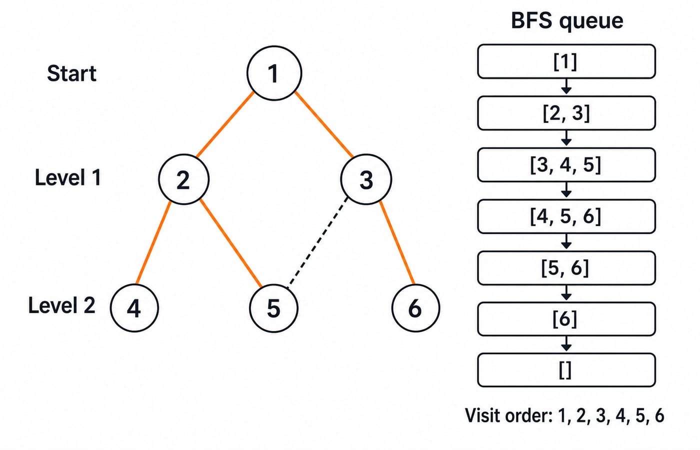
Breadth-first search explores a graph level by level using a queue, visiting all neighbours of a vertex before going deeper. Take this undirected graph, six vertices and six edges:
1 connects to 2 and 3
2 connects to 1, 4, 5
3 connects to 1, 5, 6
4 connects to 2
5 connects to 2, 3
6 connects to 3
Starting BFS at vertex 1, always taking lower-numbered neighbours first:
Visit 1. Enqueue its neighbours 2, 3.
Dequeue 2, visit it. Enqueue 4, 5.
Dequeue 3, visit it. Enqueue 6.
Dequeue and visit 4, then 5, then 6. Their neighbours are already visited.
BFS order: 1, 2, 3, 4, 5, 6. On an adjacency list, BFS visits every vertex once and scans every edge once, so it runs in O(V + E). BFS also finds the shortest path in an unweighted graph, because it reaches every vertex by the fewest edges.
DFS: depth-first search, edge classification, topological sort
Depth-first search plunges as deep as possible before backtracking, using a stack (or recursion). On the same graph from vertex 1, lower neighbours first:
From 1 go to 2, and from 2 to 4. Vertex 4's only neighbour is 2, which is already visited, so backtrack to 2 and take 5. From 5 the unvisited neighbour is 3, and from 3 the unvisited neighbour is 6.
DFS order: 1, 2, 4, 5, 3, 6. Like BFS, DFS is O(V + E) on an adjacency list.
On a directed graph, DFS classifies every edge into four types, which is a favourite exam question:
Tree edge: an edge to a newly discovered vertex.
Back edge: an edge to an ancestor still on the recursion stack. A back edge means the graph has a cycle.
Forward edge: an edge to an already-finished descendant.
Cross edge: an edge between two subtrees, neither an ancestor of the other.
Topological sort orders the vertices of a directed acyclic graph so every edge points forward. Run DFS and output vertices in decreasing order of finish time. For the dependency graph A to B, A to C, B to D, C to D, D to E, one valid topological order is A, B, C, D, E. This is exactly the "which task before which" ordering that scheduling questions use.
Shortest paths: Dijkstra, Bellman-Ford, Floyd-Warshall
For weighted graphs, the choice of algorithm turns on two questions: is any edge weight negative, and do you need distances from one source or between every pair of vertices?
Dijkstra's algorithm finds shortest paths from one source, assuming all edge weights are non-negative. It greedily settles the closest unsettled vertex, then relaxes its outgoing edges. Take a directed graph with source S and edges S to A (1), S to B (4), A to B (2), A to C (6), B to C (3).
Step | Edges relaxed | dist(A) | dist(B) | dist(C) |
|---|---|---|---|---|
Init (dist S = 0) | none | ∞ | ∞ | ∞ |
Settle S | S to A, S to B | 1 | 4 | ∞ |
Settle A | A to B, A to C | 1 | min(4, 1+2) = 3 | 1+6 = 7 |
Settle B | B to C | 1 | 3 | min(7, 3+3) = 6 |
Settle C | none left | 1 | 3 | 6 |
Final shortest distances from S: A = 1, B = 3, C = 6. Notice the direct S to B edge of weight 4 loses to the path S to A to B of weight 3, which is exactly the relaxation the greedy step catches. With a binary heap Dijkstra runs in O((V + E) log V).
Bellman-Ford handles negative edge weights and detects negative cycles by relaxing all edges V minus 1 times, at a cost of O(VE). Floyd-Warshall computes shortest paths between all pairs of vertices with three nested loops, in O(V³), and is the natural choice when you need the full distance matrix.
The non-negative condition on Dijkstra is not a technicality, and it is the failure case examiners like. Take S to A (2), S to B (5), B to A (-4). Dijkstra settles A at 2 and never revisits it, so it never discovers that S to B to A costs 5 - 4 = 1. Once a vertex is settled its distance is frozen, and a negative edge can still improve it afterwards. Bellman-Ford relaxes every edge again on each of its V minus 1 passes, so it returns 1.
How graph algorithms are tested in GATE, NET and placements
GATE CS asks for exact BFS or DFS orders on a labelled graph, the number of edges of each DFS type, whether a graph is a DAG, and single Dijkstra or Bellman-Ford relaxations. Space complexity of the matrix versus list representation is a recurring one-mark question. Solidify the underlying structure with the Data Structures learn module, which builds graphs on top of trees and queues, and drill the pattern set with our Data Structures Graphs MCQs collection of solved questions.
UGC NET Computer Science stays conceptual: match an algorithm to its complexity, identify when Dijkstra fails (negative edges), and read a traversal order. Placement interviews ask you to code BFS and DFS and reason about cycle detection, often after warming up on the binary trees and binary search trees that graphs generalise.
The short version
Fix the representation first: matrix for dense and O(1) edge checks, list for sparse and O(V + E) traversal. BFS uses a queue and finds unweighted shortest paths; DFS uses a stack, classifies edges, and gives topological order. For weighted graphs, reach for Dijkstra (non-negative), Bellman-Ford (negative edges), or Floyd-Warshall (all pairs). Hand-trace each on a small graph until the order is automatic. To work through the same sequence in order, from graph representations to DFS, BFS, topological sort and edge classification, GATE Guidance by Sanchit Sir teaches it with practice questions at each step, and the GATE CS exam category covers the rest of the paper.
Keep learning
Tree Data Structure: Types, Traversals and a Worked BST Example
Build one nine-node binary search tree, classify its shape, trace four traversals, and work through insertion, search, deletion and complexity checks.
Updated 21 Oct 20266 min readDSA & Algorithms
Graphs in Data Structures: Complete Guide with BFS, DFS and Dijkstra Worked Examples
Learn graph terminology, representations and algorithm selection by tracing one unweighted graph with BFS and DFS, then solving a weighted graph with Dijkstra.
Updated 17 Oct 20266 min readDSA & Algorithms

Physical Security and Cryptography Basics: Controls, Keys and Worked Examples
Learn how physical and cryptographic controls work together, then apply them in a four-asset server-room model and a step-by-step toy RSA example.
Updated 13 Oct 20265 min readDSA & Algorithms
Stack Data Structure: Operations, Applications and Worked Examples
Build a stack from its LIFO rule, trace array and linked-list operations, evaluate a postfix expression, and practise recursion, applications, and common traps.
Updated 8 Oct 20265 min readDSA & Algorithms