Expectation and variance questions are often lost to two quiet errors: using the variance formula backwards and failing to recognise the distribution described in words. The algebra is usually the easy part.
For an unfamiliar discrete PMF, validate its probabilities, calculate E[X] and E[X^2], then subtract in the correct order. Bernoulli, Binomial, Geometric and Poisson variables allow a faster formula-based route once the wording reveals the distribution.
Random variable, PMF, expectation and variance
A random variable assigns a numerical value to each outcome of a random experiment. For a discrete random variable X, its probability mass function, or PMF, gives P(X = x) for every possible value x.
A valid PMF has two properties:
Every probability is non-negative.
The probabilities across all possible values add to 1.
The expectation is the probability-weighted average:
E[X] = sum over x of x P(X = x).
Think of it as the centre of mass of the PMF. It need not be a value X can actually take. A die has mean 3.5 even though no face shows 3.5.
Variance measures spread around the mean:
Var(X) = E[(X - E[X])^2] = E[X^2] - (E[X])^2.
The order is load-bearing: expectation of the square minus square of the expectation. Reversing it can produce a negative answer, which variance can never be.
Fair-die expectation and variance from the definition
Let X be the number on one roll of a fair six-sided die. For k = 1, 2, ..., 6, the PMF is P(X = k) = 1/6.
First compute the mean:
E[X] = (1 + 2 + 3 + 4 + 5 + 6)/6
= 21/6 = 7/2 = 3.5.
Now compute the second moment:
E[X^2] = (1^2 + 2^2 + 3^2 + 4^2 + 5^2 + 6^2)/6
= (1 + 4 + 9 + 16 + 25 + 36)/6
= 91/6 = 15.1667 to four decimal places.
Apply the variance identity, keeping fractions exact:
Var(X) = 91/6 - (7/2)^2
= 91/6 - 49/4
= 182/12 - 147/12
= 35/12 = 2.9167 to four decimal places.
Therefore the standard deviation is
sqrt(35/12) = 1.7078 to four decimal places.
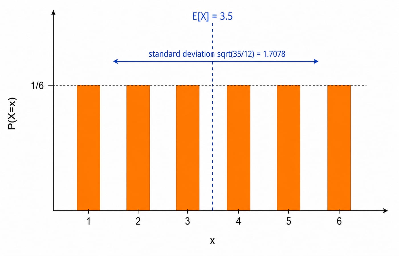
This route works for any discrete PMF: validate the probabilities, compute E[X], compute E[X^2], then subtract in the correct order.
Four named distributions GATE uses
The parameter and convention matter as much as the formula.
Distribution | PMF | E[X] | Var(X) |
|---|---|---|---|
Bernoulli(p) |
|
|
|
Binomial(n,p) |
|
|
|
Geometric(p), trials through first success |
|
|
|
Poisson(lambda) |
|
|
|
For X ~ Binomial(5, 1/2):
E[X] = np = 5(1/2) = 2.5.Var(X) = np(1-p) = 5(1/2)(1/2) = 5/4 = 1.25.P(X=2) = C(5,2)(1/2)^2(1/2)^3 = 10(1/2)^5 = 10/32 = 5/16 = 0.3125.
For a die rolled until the first 6, the success probability is p = 1/6. If X counts trials including the successful roll, then X is geometric:
E[X] = 1/(1/6) = 6.Var(X) = (1-1/6)/(1/6)^2 = (5/6)/(1/36) = (5/6)(36) = 30.
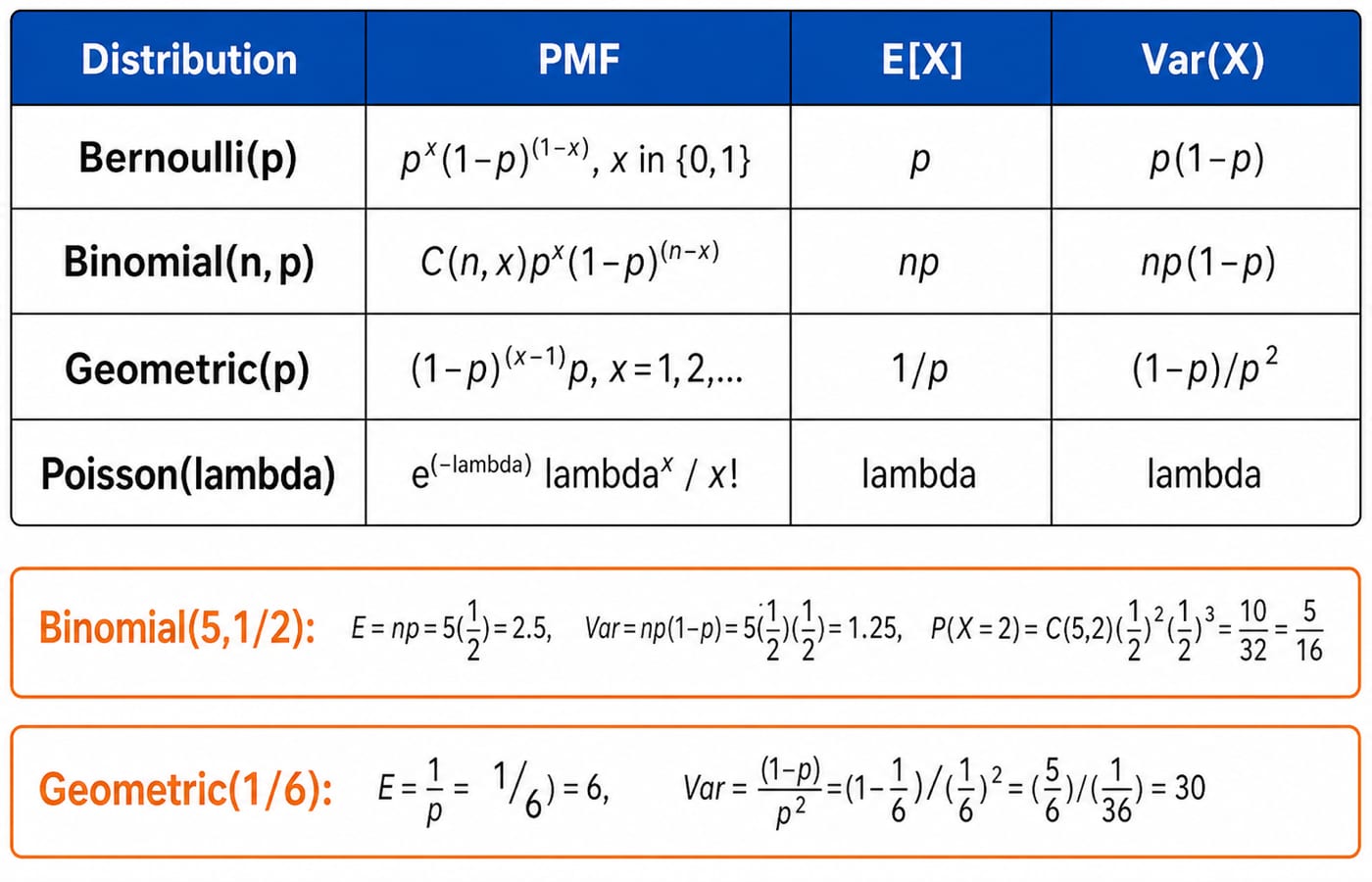
Recognition does most of the work. Fixed independent trials with a fixed success probability and a count of successes suggest Binomial. Trials until the first success suggest Geometric. A count of events in a fixed interval often signals Poisson.
Linearity and variance scaling shortcuts
Linearity of expectation says
E[aX + b] = aE[X] + b
and
E[X + Y] = E[X] + E[Y].
The second identity holds even when X and Y are dependent. For two fair dice X and Y, the expected sum is immediately
E[X+Y] = E[X] + E[Y] = 3.5 + 3.5 = 7.
No joint PMF is needed for that expectation.
Do not copy that independence-free rule to variance. In general, Var(X+Y) = Var(X) + Var(Y) + 2Cov(X,Y). You may add variances directly only when the covariance is zero.
Variance transforms differently:
Var(aX+b) = a^2 Var(X).
The constant b disappears, while the multiplier is squared. For the fair die,
Var(2X+5) = 2^2(35/12) = 4(35/12) = 140/12 = 35/3.
One more rearrangement saves time:
E[X^2] = Var(X) + (E[X])^2.
If a question supplies the mean and variance, it has effectively supplied the second moment too.
Expectation and variance traps
Variance sign: use E[X^2] - (E[X])^2, never the reverse.
Geometric convention: counting trials through the first success gives mean 1/p. Counting failures before the first success starts at zero and gives mean (1-p)/p. Read the random variable's definition.
Binomial variance: the mean is np, but the variance is np(1-p). Do not replace the variance with the mean simply because both formulas begin with np.
Variance versus standard deviation: variance is in squared units. Standard deviation is its non-negative square root.
Constants: Var(c)=0, and adding a constant does not change variance. Multiplying by a scales variance by a^2, not a.
If binomial coefficients are slowing you down, revise Permutations and Combinations for GATE CS. For conditional setups and posterior probability, continue with Probability for GATE CS: Conditional Probability and Bayes.
How GATE tests random variables
The recurring shapes are: compute mean or variance from a PMF, identify a named distribution, recover a second moment, or combine a transformation with a standard result. A two-mark question often hides a simple scaling rule behind a familiar distribution.
For the exact Probability and Statistics wording under Engineering Mathematics, check the current syllabus on the official GATE portal of the organising IIT. Do not rely on an old coaching list for official scope.
KnowledgeGate has more than 500 probability and statistics questions. For expectation and variance practice, use mixed sets so that you must first identify the distribution and only then select the formula.
The short version and next step
Memorise the four-row table, keep Var(X) = E[X^2] - (E[X])^2 in the correct order, and try linearity before building a joint distribution.
The Engineering Mathematics course provides the structured track, while the GATE category connects this chapter with the wider exam preparation path. Then solve enough mixed numericals that recognising Bernoulli, Binomial, Geometric and Poisson becomes automatic.