Backtracking and branch and bound both search a state-space tree, so memorised definitions can blur together in an exam. The real question is what makes each method reject a branch and how that changes the nodes explored. Trace one small tree carefully, and the distinction becomes mechanical rather than verbal.
1. One tree, two prunings
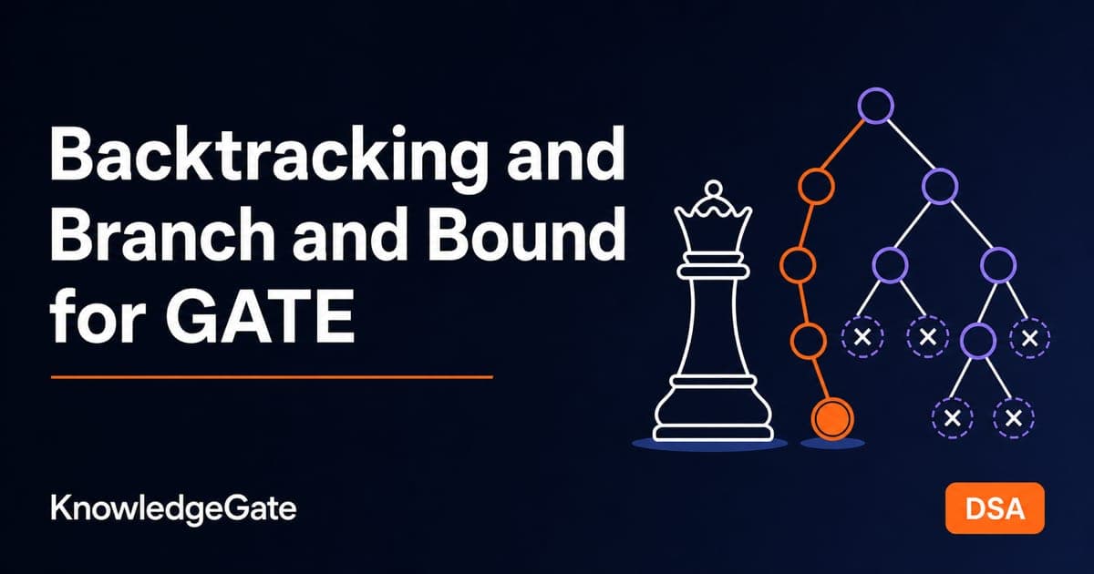
A state-space tree represents choices. Its root is the empty partial solution, each edge adds one decision, and each node records the decisions made so far. Both methods avoid exploring every complete combination, but they prune for different reasons.
Backtracking is mainly used for feasibility or enumeration. A partial solution that already violates a constraint cannot become valid later, so the algorithm stops extending it. N-Queens, graph colouring, Hamiltonian cycles and sum of subsets are standard examples.
Branch and bound is used for optimisation. A node carries a bound on the best objective value its entire subtree could possibly reach. If that best case cannot improve the best complete solution already found, called the incumbent, the subtree is discarded.
This is the clean exam sentence: backtracking prunes an infeasible partial solution, while branch and bound prunes a feasible or undecided branch that cannot become optimal.
2. Backtracking in detail
Backtracking builds a solution vector one component at a time. At each node it chooses a candidate value, checks whether the partial vector is promising, and recurses only if the constraints still hold. When no candidate works, control returns to the previous level and tries its next choice. That return is the backtrack.
The usual traversal is depth-first. Only the current path and the information needed to undo a choice must remain active, so working memory tracks tree depth rather than every live node. This is different from a breadth-first branch-and-bound strategy, which may keep many live nodes at once.
A useful discipline is to write the constraint before drawing the tree. For N-Queens, a new queen must avoid every used column and every occupied diagonal. Without that test written down, students often prune by visual intuition and miscount a node.
3. Fully worked example: 4-Queens
Place one queen in every row of a 4 by 4 board so that no two queens share a column or diagonal. Represent a placement as (row, column). Queens at (r1, c1) and (r2, c2) share a diagonal exactly when |r1 - r2| = |c1 - c2|. Each tree level chooses the column for the next row.
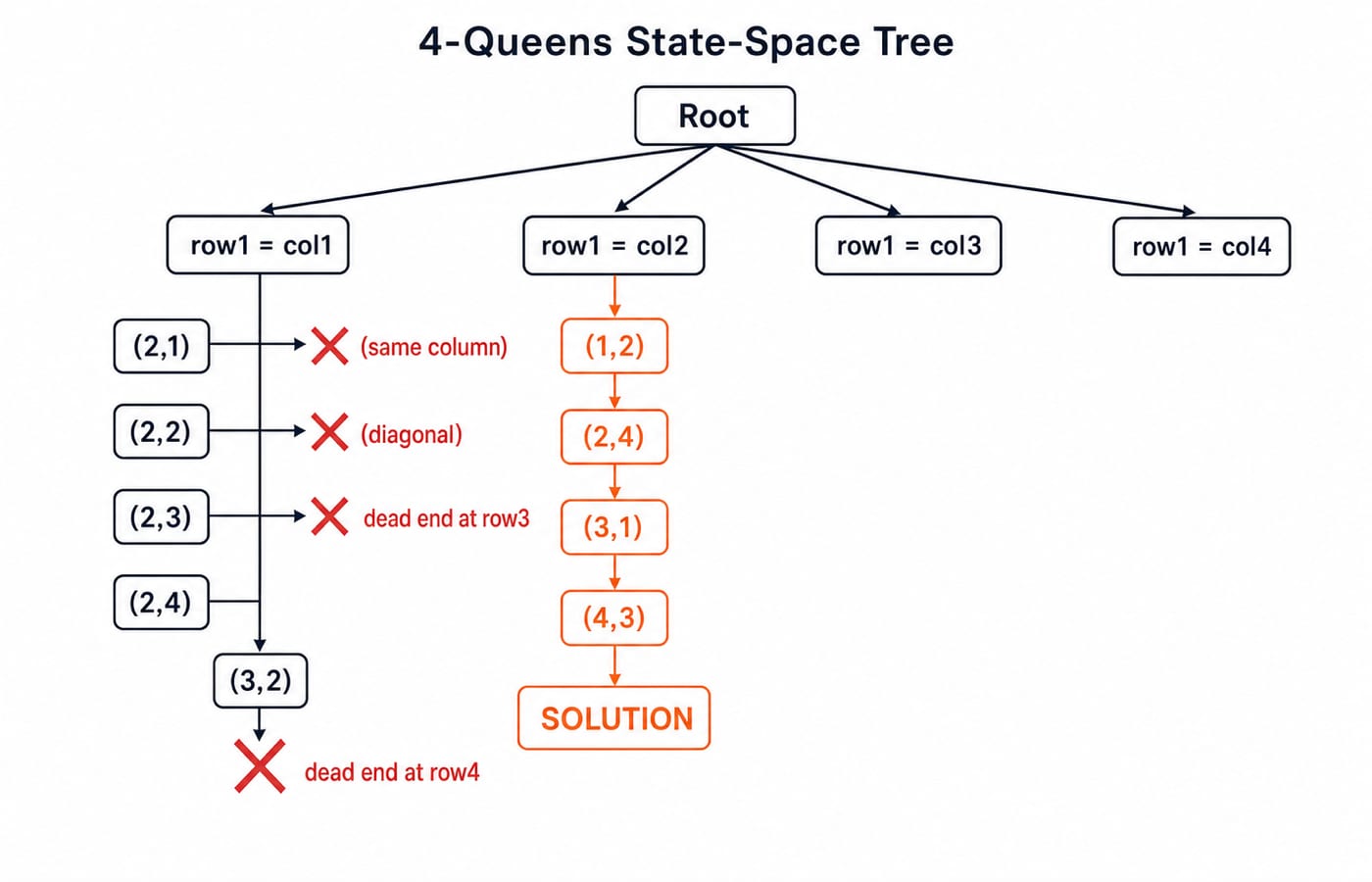
Start with row 1, column 1.
Row 2, column 1 fails because the column repeats. Column 2 fails because the row difference and column difference are both 1.
Row 2, column 3 is safe, giving
(1,1), (2,3). For row 3, column 1 repeats column 1, column 2 is diagonal to(2,3), column 3 repeats column 3, and column 4 is also diagonal to(2,3). This branch has no child.Backtrack to row 2 and try column 4. Row 3, column 2 is safe, giving
(1,1), (2,4), (3,2). Row 4 then has no safe column. Column 1 repeats the first queen's column, column 2 repeats the third queen's column, column 3 is diagonal to(3,2), and column 4 repeats the second queen's column.
The entire row 1, column 1 subtree has now failed.
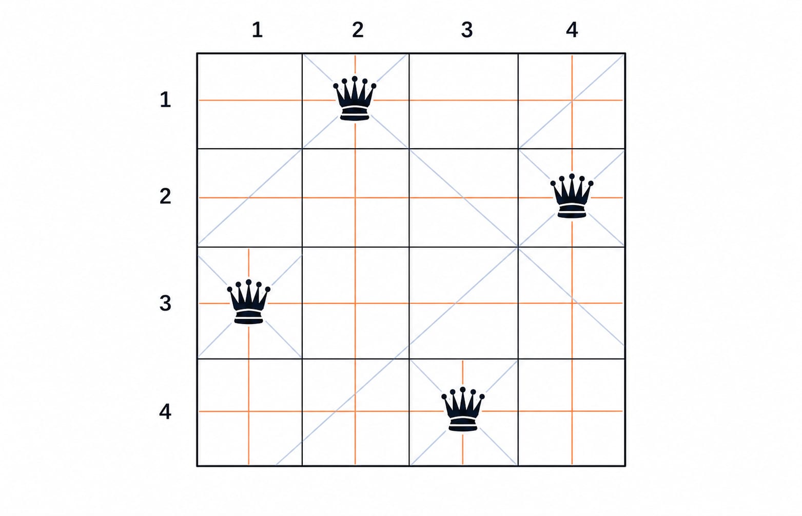
Try row 1, column 2. Row 2, column 4 is safe. Row 3, column 1 is safe because its column is unused and its diagonal differences do not equal the row differences against either earlier queen. Row 4, column 3 is then safe. The first complete solution is (1,2), (2,4), (3,1), (4,3).
Reflecting that board across its vertical axis gives (1,3), (2,1), (3,4), (4,2). These are the only two solutions to 4-Queens.
4. Counting the state-space tree
If every row could independently choose any of four columns and constraints were ignored, there would be 4 x 4 x 4 x 4 = 4^4 = 256 complete leaves. If only the no-repeated-column rule were applied, each complete placement would be a permutation, giving 4! = 4 x 3 x 2 x 1 = 24 leaves. The diagonal test cuts this set further, and only two complete solutions survive.
Do not confuse leaves with all generated nodes. If a question asks for nodes generated, count the root and every partial placement the stated algorithm actually reaches, according to its own convention. A branch pruned at row 3 contributes the nodes reached before the failure, but it contributes no row 4 descendants. There is no universal shortcut because traversal order, constraint-check timing and the question's counting convention determine the total.
5. Branch and bound and the bounding function
Branch and bound keeps live nodes and selects one to expand. FIFO selection behaves breadth-first, LIFO behaves depth-first, and least-cost or LC selection expands the most promising bound first. The selection rule changes order, while the bound decides whether a subtree remains worth exploring.
Consider 0/1 knapsack with capacity 15. Items are sorted by value-to-weight ratio: A(w=2,v=10), B(w=3,v=12), C(w=5,v=18) and D(w=7,v=21). Their ratios are 5, 4, 3.6 and 3, so this is the required order.
At the root, compute an optimistic upper bound by filling the remaining capacity greedily and allowing a fraction of the final item:
Take A, B and C fully. Weight used is
2 + 3 + 5 = 10, and value is10 + 12 + 18 = 40.Capacity remaining is
15 - 10 = 5.Only
5/7of D fits in the fractional relaxation. Its bound contribution is21 x 5/7 = 15.The root upper bound is therefore
40 + 15 = 55.
The fractional item does not become a legal 0/1 solution. It deliberately overestimates what a descendant might achieve, which makes 55 a safe upper bound. A legal solution chooses B, C and D: its weight is 3 + 5 + 7 = 15 and its value is 12 + 18 + 21 = 51, so 51 becomes the incumbent. Now inspect the node that includes A and excludes B. Even after adding C and D, its maximum possible value is 10 + 18 + 21 = 49 at weight 2 + 5 + 7 = 14. Since 49 cannot beat 51, that node is pruned. This is how the bound becomes a decision: 55 is the optimistic root ceiling, not a feasible 0/1 value. A related contrast is greedy algorithms explained: greedy filling creates the bound here, but it does not by itself solve the 0/1 problem.
6. Backtracking versus branch and bound, and how GATE tests this
Feature | Backtracking | Branch and bound |
|---|---|---|
Main goal | Find or enumerate feasible solutions | Find an optimal solution |
Pruning test | Partial choice violates a constraint | Best possible objective cannot beat incumbent |
Typical traversal | Depth-first | FIFO, LIFO or least-cost |
Classic problems | N-Queens, colouring, Hamiltonian cycle | Knapsack, travelling salesperson, assignment |
GATE can ask you to count generated nodes in a small state-space tree, identify FIFO, LIFO or LC selection, or calculate a node's bound. Two traps matter. Backtracking normally uses depth-first search, and neither method guarantees fewer expansions than exhaustive search in the worst case.
About 1,100 Algorithms questions are available in KnowledgeGate for practice around these patterns. Confirm the current Algorithms syllabus and any weightage claim on the official GATE portal. For the broader design-method comparison, dynamic programming explained shows how overlapping subproblems lead to a different kind of reuse. The GATE CS catalogue places all three methods in the wider subject map.
7. The short version and your next step
Both methods search a state-space tree. Backtracking rejects a partial solution when a constraint fails. Branch and bound rejects a subtree when its best possible objective cannot beat the incumbent. In 4-Queens, constraint checks leave exactly two solutions; in the knapsack relaxation above, the root upper bound is 55.
Build the full Algorithms sequence with GATE Guidance by Sanchit Sir, then use the GATE Test Series to practise tree traces and bounds under exam timing.