

Probability Distributions for Machine Learning: Match Bernoulli, Binomial, Normal and Poisson to Data
Learn a reusable way to match binary outcomes, grouped successes, event counts and continuous residuals to a defensible probability model.
KnowledgeGate Team
Exam prep & CS education
Updated 13 Nov 20266 min read

The formulas are usually not the difficult part. The real difficulty is deciding what one random variable represents and which assumptions the data can support. In machine learning, we usually model a target or residual conditional on features, such as P(Y | X). We do not require every input column to follow the selected distribution. Choose among Bernoulli, Binomial, Poisson and Normal models by checking support, exposure or fixed trials, independence, and finally the diagnostics.
Probability distributions for machine learning start with the target's support
A probability distribution describes the possible values of a target and assigns probabilities to them. Start by defining what one target value means. Is it one binary result, successes in a fixed number of trials, an event count over an exposure, or a continuous residual around a predicted mean?
Distribution | Possible values | Core parameters | Assumptions to check | ML use |
|---|---|---|---|---|
Bernoulli | Y in {0,1} | p | One binary outcome, correct conditional probability | Binary classification |
Binomial | K in {0,...,n} | n, p | Fixed n, common p, conditional independence | Grouped success counts |
Poisson | K in {0,1,2,...} | lambda | Stable rate for a stated exposure, suitable event independence | Count regression |
Normal | Y in all real numbers | mu, sigma^2 | Continuous residuals, symmetry, stable spread | Regression with squared error |
Explore Skill Development Courses for a broader route from these statistical foundations to applied technical practice. In the wider model-choice context, Approaches to AI explains other ways an intelligent system can represent and act on a problem.
The data type narrows the candidates. It does not finish the choice. Independence, equal probability, a stable rate and residual shape decide whether the candidate is defensible.
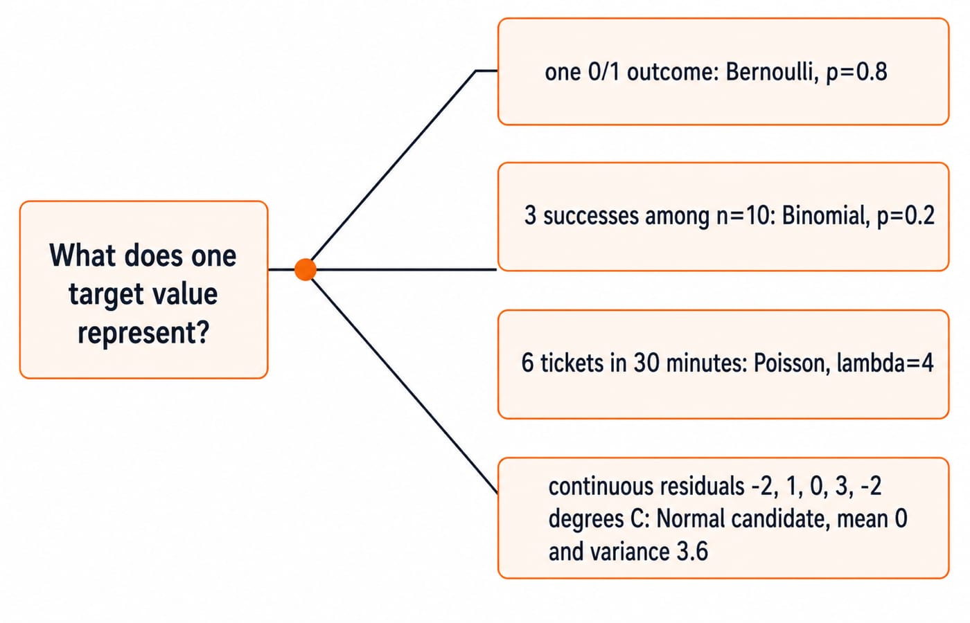
Bernoulli distribution models one binary outcome
For Y ~ Bernoulli(p), P(Y=1)=p and P(Y=0)=1-p. One row might represent a conversion, churn event, fraud flag or pass/fail label. A classifier can estimate a different p_i=P(Y_i=1 | X_i) for every row. The outcomes are still Bernoulli even though their predicted probabilities differ.
Take labels y=[1,0,1,1] and predictions p=[0.8,0.3,0.6,0.9]. For a positive label, use p_i; for a negative label, use 1-p_i. The likelihood is
Likelihood = 0.8 x (1 - 0.3) x 0.6 x 0.9
= 0.8 x 0.7 x 0.6 x 0.9
= 0.3024.
Therefore, the total negative log-likelihood is -ln(0.3024), approximately 1.1960. The mean binary cross-entropy is 1.1960/4, approximately 0.2990. A confident correct prediction puts a factor close to one in the likelihood and contributes a small loss. A confident wrong prediction puts a factor close to zero in it and contributes a large loss.
Bernoulli describes each individual 0/1 outcome. A sum of suitable Bernoulli trials gives a count, but that count is not automatically Binomial.
Binomial distribution needs a fixed number of comparable trials
Use K ~ Binomial(n, p) when there are exactly n trials, two outcomes per trial, a common success probability p, and independence conditional on the model. “Did this user convert?” is Bernoulli. “How many of 10 comparable users converted?” can be Binomial.
For n=10, p=0.2 and K=3,
P(K = 3) = C(10, 3) x (0.2)^3 x (0.8)^7
= 120 x 0.008 x 0.2097152
= approximately 0.2013.
Its expected count is E[K]=np=10 x 0.2=2. Its variance is Var(K)=np(1-p)=10 x 0.2 x 0.8=1.6.
If the 10 users have materially different probabilities, the ordinary equal-p assumption fails. Keep the row-level Bernoulli likelihoods, or recognise that their sum follows a Poisson-binomial distribution. For a refresher on events, conditioning, Bayes' rule and expectation, read Probability for GATE CS.
Poisson distribution models event counts over exposure
For K ~ Poisson(lambda), possible counts are 0,1,2,..., while both the mean and variance equal lambda. It suits arrivals, defects, claims or tickets per unit of time, area or traffic exposure when there is no fixed trial ceiling.
Suppose a service desk averages lambda=4 tickets per 30 minutes. Then
P(K = 6) = e^(-4) x 4^6 / 6!
= e^(-4) x 4096 / 720
= approximately 0.1042.
If the rate is stable and exposure doubles, the mean also doubles. The corresponding one-hour mean is 8, not 4.
Poisson regression predicts a positive conditional mean lambda(X), commonly through a log link. Exposure must be represented when rows cover different durations or populations. Poisson is not defined as “Binomial with a large n”. A Poisson approximation to the Binomial needs specific rare-event conditions.
Normal distribution is usually an assumption about continuous residuals
A useful regression statement is Y | X ~ Normal(mu(X), sigma^2). The Normal assumption concerns errors around the conditional mean. It does not require every feature, or even the marginal target histogram, to look Normal.
Consider temperature-sensor residuals [-2,1,0,3,-2] degrees C. Their mean is (-2+1+0+3-2)/5=0. The squared residuals are [4,1,0,9,4], so the sum of squared errors is 18. Thus,
MSE = estimated variance = 18 / 5 = 3.6,
Estimated sigma = sqrt(3.6), approximately 1.897 degrees C.
For fixed variance, maximising the Gaussian likelihood is equivalent to minimising squared error. Check the assumption through residual plots: look for symmetry around zero, roughly stable spread across predictions, and limited tail outliers. Heavy tails or changing variance can make uncertainty estimates unreliable even when point predictions remain useful.
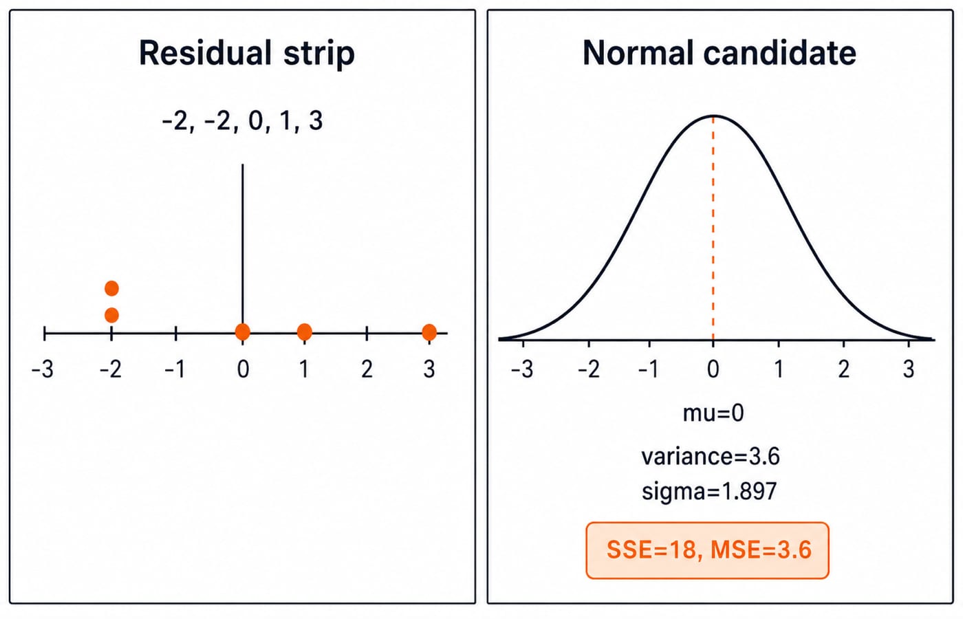
Distribution assumptions determine the loss, then diagnostics test the fit
The assumed target distribution leads to the training objective. Bernoulli leads to binary cross-entropy. Grouped Binomial data leads to Binomial negative log-likelihood. Poisson counts lead to Poisson log-likelihood or deviance. A Normal model with fixed variance leads to squared error. A loss function is therefore an assumption about how targets vary, not merely a software setting.
Now inspect observed counts [0,1,1,2,8,12]. Their mean is 24/6=4. The squared deviations from 4 are [16,9,9,4,16,64], with total 118. Their population variance is
Population variance = 118 / 6, approximately 19.67.
This variance is far above the Poisson mean of 4, which signals overdispersion. Ask whether rates differ across rows, events cluster, or a negative-binomial model would fit better.
Use this trap checklist:
Never choose a distribution from the histogram alone.
Never confuse probability with likelihood.
Never treat correlated repeated observations as independent.
Never use a Normal model for an untransformed non-negative count.
Never ignore changing exposure.
Probability distribution questions test assumptions before arithmetic
These are representative assessment or interview scenarios, not official previous-year questions:
One loan default flag: Bernoulli, because one observation is binary.
Seven defaults among 50 comparable independent loans with common p: Binomial, because the trial count is fixed and the trials share p.
Defects per metre of fabric with metres recorded: Poisson with exposure, because the target is an event count over measured material.
Symmetric measurement error around a calibrated prediction: Normal is a candidate because the residual is continuous and centred around the prediction.
Test the boundaries too. Varying per-customer probabilities break the simple Binomial model. A count variance far above its mean challenges the Poisson model. Name the failed assumption first, then consider an alternative. That reasoning matters more than memorising four mass or density formulas.
The short version: match the random variable, then verify the assumptions
Define one target value, identify its support and exposure, state the independence or residual assumptions, fit the corresponding likelihood, and inspect whether the observed errors or counts contradict it.
Bernoulli is one binary outcome, Binomial is successes in fixed comparable trials, Poisson is an event count per exposure, and Normal is a continuous value or residual around a mean. If you want a structured route through applied AI and machine learning, the Artificial Intelligence (AI) course is the relevant next step in the course catalog.
Keep learning

Conditional Probability for Machine Learning: Bayes' Rule with a Worked Classifier Example
Follow one hypothetical classifier from conditional probability to Bayes' posterior. Verify the answer with natural frequencies, compare precision with recall, and see exactly what a stricter threshold changes.
Updated 10 Nov 20266 min readML & Data Science

Hypothesis Testing for Machine Learning: Separate Signal from Sampling Noise in Model Comparisons
Learn one complete paired-model comparison, from a 2 by 2 prediction table and exact p-value to effect size, confidence interval, test choice, and leakage checks.
Updated 17 Nov 20266 min readML & Data Science

GATE DA Machine Learning Revision Map: From Probability to Neural-Network Calculations
Connect five machine-learning note sets through four worked problems and a complete neural-network forward pass, with a focused 90-minute revision loop.
Updated 5 Nov 20265 min readML & Data Science

Covariance and Correlation for Machine Learning: Read Feature Relationships Correctly
Calculate covariance and Pearson correlation by hand, then see how units, influential points and nonlinear patterns change what the numbers mean.
Updated 14 Nov 20266 min readML & Data Science