

Covariance and Correlation for Machine Learning: Read Feature Relationships Correctly
Calculate covariance and Pearson correlation by hand, then see how units, influential points and nonlinear patterns change what the numbers mean.
KnowledgeGate Team
Exam prep & CS education
Updated 14 Nov 20266 min read

A dataframe can show two columns rising together, yet a raw covariance is hard to compare and a correlation coefficient can hide curves or outliers. Neither number explains why a relationship exists. In the five-learner table below, population covariance is 10.2 test-points and Pearson r is 0.9964; changing units leaves r unchanged, one influential sixth row flips it to -0.4205, and A versus A^2 shows why r=0 can hide exact dependence. Read linear direction and strength without confusing correlation with causation, exact redundancy or general dependence.
Covariance and correlation answer related but different questions
Covariance is the average paired movement around two feature means. It is positive when above-mean values tend to pair with above-mean values, negative when one feature tends to be above its mean as the other is below, and near zero when positive and negative cross-products cancel. Its magnitude carries both features' units, so it is not a universal strength scale.
Pearson correlation standardises covariance:
r = cov(X,Y) / (sd_X × sd_Y)
When both standard deviations are non-zero, r is unitless, lies between -1 and 1, and measures the direction and strength of a linear relationship. Labels such as weak or strong need context, sample size and a scatter plot. For broader applied learning, use Skill Development Courses.
Centre the feature table and compute covariance by hand
Let X be practice tests completed and Y be mock score in points.
Learner | X: practice tests completed | Y: mock score (points) |
|---|---|---|
S1 | 1 | 52 |
S2 | 2 | 56 |
S3 | 3 | 63 |
S4 | 4 | 67 |
S5 | 5 | 72 |
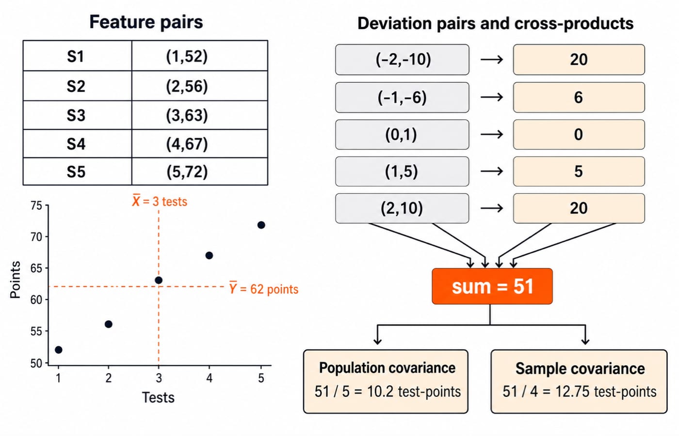
mean_X = (1+2+3+4+5)/5 = 3 tests, while mean_Y = (52+56+63+67+72)/5 = 310/5 = 62 points.
Learner |
|
| Cross-product |
|---|---|---|---|
S1 | -2 | -10 | 20 |
S2 | -1 | -6 | 6 |
S3 | 0 | 1 | 0 |
S4 | 1 | 5 | 5 |
S5 | 2 | 10 | 20 |
Sum | 51 |
S1 and S2 are below both means, while S4 and S5 are above both, so their paired deviations contribute positive products. Treating the five learners as the complete illustrative batch gives population covariance cov_pop(X,Y) = 51/5 = 10.2 test-points. If they are a sample used to estimate a wider population covariance, use the sample denominator once: cov_sample(X,Y) = 51/(5-1) = 51/4 = 12.75 test-points. Never mix these denominators. Descriptive Statistics for ML: Mean, Variance, IQR and Robust Summaries explains one-feature centre, spread and robust scaling. Covariance and correlation instead measure paired linear movement.
Pearson correlation removes the units, not the assumptions
Continue with the same deviations:
sum (X_i-3)^2 = 4+1+0+1+4 = 10
sum (Y_i-62)^2 = 100+36+1+25+100 = 262
Using population denominators, var_X = 10/5 = 2 and sd_X = sqrt(2) = 1.4142 tests. Likewise, var_Y = 262/5 = 52.4 and sd_Y = sqrt(52.4) = 7.2388 points. Therefore:
r = 10.2 / (1.4142 × 7.2388) = 0.9964
The cancellation-friendly calculation reaches the same result:
r = 51 / sqrt(10 × 262) = 51 / sqrt(2620) = 0.9964
Sample covariance and sample standard deviations also produce the same r because their common n-1 factors cancel when used consistently. The five plotted points have a very strong positive linear association. This does not show that one extra practice test causes a fixed score gain, guarantees a result, or describes learners outside this tiny illustrative batch.
Units change covariance; a correlation matrix can expose exact duplication
Define M = 60X, so practice minutes are [60,120,180,240,300] and mean_M = 180. Multiplying X by 60 multiplies its population covariance with Y by 60:
cov_pop(M,Y) = 60 × 10.2 = 612 minute-points
Using the unrounded value before display, sd_M = 60 × sqrt(2) = 84.8528 minutes. Thus r(M,Y) = 612 / (84.8528 × 7.2388) = 0.9964 after rounding.
X | Y | M | |
|---|---|---|---|
X | 1 | 0.9964 | 1 |
Y | 0.9964 | 1 | 0.9964 |
M | 1 | 0.9964 | 1 |
A correlation matrix is symmetric, and each diagonal entry is one for a non-constant feature. X and M are redundant because the known construction M=60X makes them exact copies in different units. X and Y sit close to a line in five rows, but 0.9964 does not prove semantic duplication. Linear Algebra for GATE CS provides the adjacent matrix foundation.
A scatter plot reveals what one coefficient hides
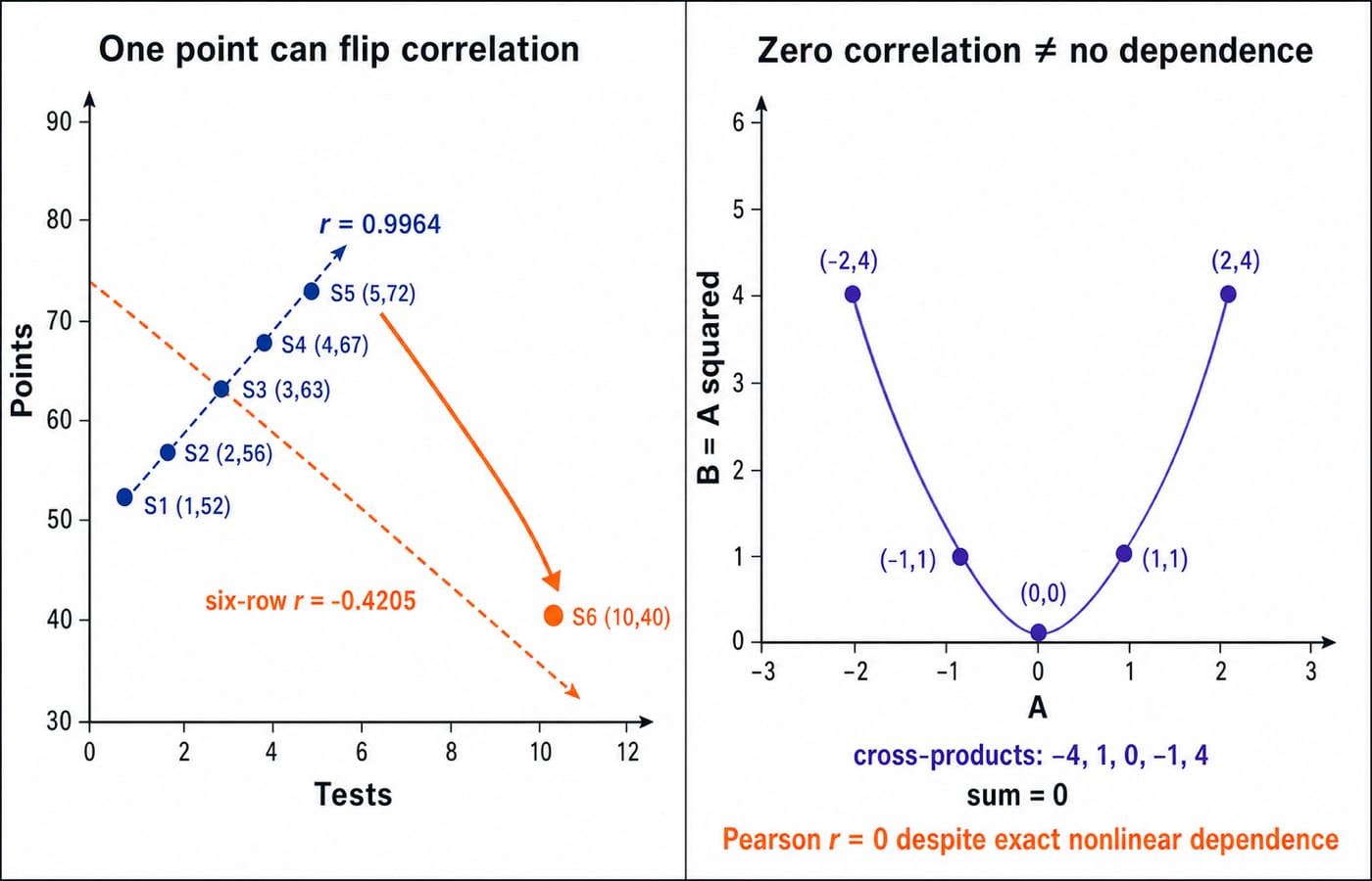
First plot (1,52), (2,56), (3,63), (4,67) and (5,72) before interpreting r=0.9964. Now add the influential learner S6=(10,40). Across all six rows:
mean_X = 25/6 = 4.1667mean_Y = 350/6 = 58.3333cross-product sum
= -77.3333X squared-deviation sum
= 50.8333Y squared-deviation sum
= 665.3333cov_pop(X,Y) = -77.3333/6 = -12.8889r = -77.3333 / sqrt(50.8333 × 665.3333) = -0.4205
One high-leverage point far to the right and below the original trend changes a five-row near-perfect positive coefficient into a moderate negative coefficient. Do not automatically dismiss S6 as bad data. Check its units, collection process and learner context before correcting, retaining, segmenting or choosing a robust method.
Now take A=[-2,-1,0,1,2] and B=A^2=[4,1,0,1,4]. Their means are 0 and 2. The centred cross-products are -4, 1, 0, -1, 4, which sum to 0. Population covariance and Pearson r are both 0, although B is determined exactly by A. Zero linear correlation does not imply independence or no relationship.
Correlation is not causation, and high correlation is not an automatic delete rule
Prior mastery, motivation, course track, study time or test difficulty could affect practice tests, mock scores or both. This observational table cannot isolate the effect of completing another test. A causal claim needs a defensible design and assumptions beyond a coefficient.
For feature selection, follow a sequence:
Verify each column's name and measurement.
Inspect missingness and the same-row scatter.
Check for linearity and subgroup patterns.
Identify deterministic transforms such as
M=60X.Compare model validation with and without the feature.
Keep one of X and M unless the system documents a reason to retain both. Do not delete Y merely because r(X,Y)=0.9964 in five rows. Calculate correlation-based feature selection only from training data, then apply the selected feature set unchanged to validation and test data. Implement the calculation through the Python Course.
Assessment and interview checks test definitions, arithmetic and judgement
Representative checks, not official PYQs:
Add 10 to each
Y?
cov_pop stays 10.2; r stays 0.9964.
Scale
Xby 60?
Covariance becomes 612; r stays unchanged.
Multiply one feature by
-1?
The sign of r flips.
Correlate
XwithC=[7,7,7,7,7]?
Undefined, because sd_C=0.
What does
AversusA^2show?
r=0 does not prove independence.
Trap | Repair |
|---|---|
Raw products | Centre both features. |
| It is sample; population is |
Covariance treated as unitless strength | Keep compound units. |
| Keep precision; inspect why. |
Category codes | Codes do not establish order. |
Different missing-value subsets used silently | Disclose pairwise rows. |
S6 deleted immediately | Investigate it first. |
"Correlation proves causation" | Require a causal design. |
Use four questions: Which rows and units produced the number? Is the scatter linear? Do outliers or subgroups control it? What mechanism, transformation or causal design explains it?
Covariance and correlation: the short version and next step
Centre paired values.
Sum their cross-products.
Choose and label the population or sample denominator.
Standardise by both standard deviations for Pearson
r.Inspect the scatter plot and data-generating context.
For the five learners, cov_pop(X,Y)=10.2 test-points and r=0.9964. After S6, r=-0.4205. For A and A^2, r=0 despite exact dependence. Now recompute the cross-product sum 51 and explain why M=60X changes covariance but not correlation. For a structured route through the broader topic, use the Artificial Intelligence (AI) course.
Keep learning

Hypothesis Testing for Machine Learning: Separate Signal from Sampling Noise in Model Comparisons
Learn one complete paired-model comparison, from a 2 by 2 prediction table and exact p-value to effect size, confidence interval, test choice, and leakage checks.
Updated 17 Nov 20266 min readML & Data Science

Probability Distributions for Machine Learning: Match Bernoulli, Binomial, Normal and Poisson to Data
Learn a reusable way to match binary outcomes, grouped successes, event counts and continuous residuals to a defensible probability model.
Updated 13 Nov 20266 min readML & Data Science

Conditional Probability for Machine Learning: Bayes' Rule with a Worked Classifier Example
Follow one hypothetical classifier from conditional probability to Bayes' posterior. Verify the answer with natural frequencies, compare precision with recall, and see exactly what a stricter threshold changes.
Updated 10 Nov 20266 min readML & Data Science

GATE DA Machine Learning Revision Map: From Probability to Neural-Network Calculations
Connect five machine-learning note sets through four worked problems and a complete neural-network forward pass, with a focused 90-minute revision loop.
Updated 5 Nov 20265 min readML & Data Science