

Conditional Probability for Machine Learning: Bayes' Rule with a Worked Classifier Example
Follow one hypothetical classifier from conditional probability to Bayes' posterior. Verify the answer with natural frequencies, compare precision with recall, and see exactly what a stricter threshold changes.
KnowledgeGate Team
Exam prep & CS education
Updated 10 Nov 20266 min read

A model can be 90% sensitive while most positive predictions are wrong. That sounds contradictory only when we reverse a conditional probability or ignore the base rate. In a hypothetical evaluation of 10,000 records, 2% prevalence, 90% sensitivity, and a 5% false-positive rate produce 670 positive predictions, but only 180 are true positives. The posterior is about 26.9%. Sensitivity conditions on actual positives, while precision conditions on predicted positives; Bayes' rule and the count table reconcile the two.
1. Conditional probability changes the reference group
Conditional probability restricts the cases we are looking at:
P(A | B) = P(A intersection B) / P(B), provided P(B) > 0.
The vertical bar means "given". It is not division or proof that B causes A.
Here, D means the condition is actually present, not D means it is absent, + means the model predicts positive, and - means it predicts negative. Then P(+ | D) is sensitivity, the share of actual positives caught by the model. By contrast, P(D | +) asks what share of positive predictions truly belong to class D.
Different reference groups give different denominators and values. Probabilistic classifiers can output a score without that score being a calibrated probability.
2. Bayes' rule turns a forward model into a posterior
Write the joint event two ways:
P(D intersection +) = P(+ | D)P(D)
P(D intersection +) = P(D | +)P(+)
Equating them and rearranging gives:
P(D | +) = P(+ | D)P(D) / P(+)
For two classes, split the evidence into both routes to a positive prediction:
P(+) = P(+ | D)P(D) + P(+ | not D)P(not D)
Here P(D) is the prior, the next two terms are the likelihood and competing-class likelihood, P(+) is the evidence, and P(D | +) is the posterior. Likelihood fixes the observed prediction and compares class hypotheses. It is not the posterior. Probability for GATE CS covers conditional probability, Bayes' theorem and expectation for the wider exam toolkit; the classifier here isolates base-rate inversion and verifies it with counts. The earlier GATE DA Machine Learning Revision Map uses a separate two-feature Naive Bayes calculation inside a broader revision sequence; this worked example instead follows one operating point through natural frequencies, confusion-matrix metrics, a threshold change and odds.
3. Build the classifier example from 10,000 records
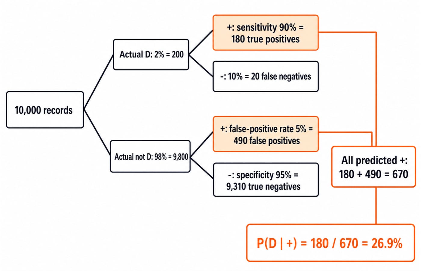
Take exactly 10,000 records. With P(D) = 0.02, 200 are actually positive and 9,800 are actually negative. Sensitivity is P(+ | D) = 0.90. Specificity is P(- | not D) = 0.95, so the false-positive rate is 1 - 0.95 = 0.05.
Actual class and prediction | Calculation | Count | Meaning |
|---|---|---|---|
|
| 180 | True positives |
|
| 20 | False negatives |
|
| 490 | False positives |
|
| 9,310 | True negatives |
Predicted positives total 180 + 490 = 670; predicted negatives total 20 + 9,310 = 9,330. These hypothetical counts do not represent measured performance for any real model, disease, institution or product.
4. Work Bayes' rule and check it against the counts
Substitute the exact rates:
P(D | +) = (0.90 x 0.02) / [(0.90 x 0.02) + (0.05 x 0.98)]
The numerator is 0.018, the false-positive contribution is 0.049, and the evidence is 0.018 + 0.049 = 0.067. Thus:
P(D | +) = 0.018 / 0.067 = 0.268656..., or about 26.9%.
Now check it with natural frequencies:
180 / (180 + 490) = 180 / 670 = 0.268656...
The routes agree because the tree scales the probability calculation to 10,000. P(+ | D) = 90% asks how many actual positives are caught. P(D | +) = 26.9% asks how many positive predictions are correct. The 2% prior leaves 49 times as many negatives as positives, so the 5% false-positive rate creates 490 false alarms against 180 true positives.
5. The posterior is precision, not recall or accuracy
The confusion-matrix counts give four different metrics:
Recall or sensitivity:
180 / 200 = 90%Specificity:
9,310 / 9,800 = 95%Precision or positive predictive value:
180 / 670 = 26.9%Accuracy:
(180 + 9,310) / 10,000 = 94.9%
For this population and threshold, the Bayes posterior after + is precision, not recall or accuracy.
Accuracy hides class imbalance. Predicting every record as negative gets 9,800 of 10,000 correct, or 98%, yet catches none of the 200 positives. Therefore, 94.9% accuracy alone cannot establish usefulness. Evaluation must reflect both error costs.
A + label does not give every flagged record a 26.9% probability. That is the aggregate posterior for this population, rates, and threshold. Calibrated individual scores may differ.
6. A threshold change alters likelihoods, not the prior
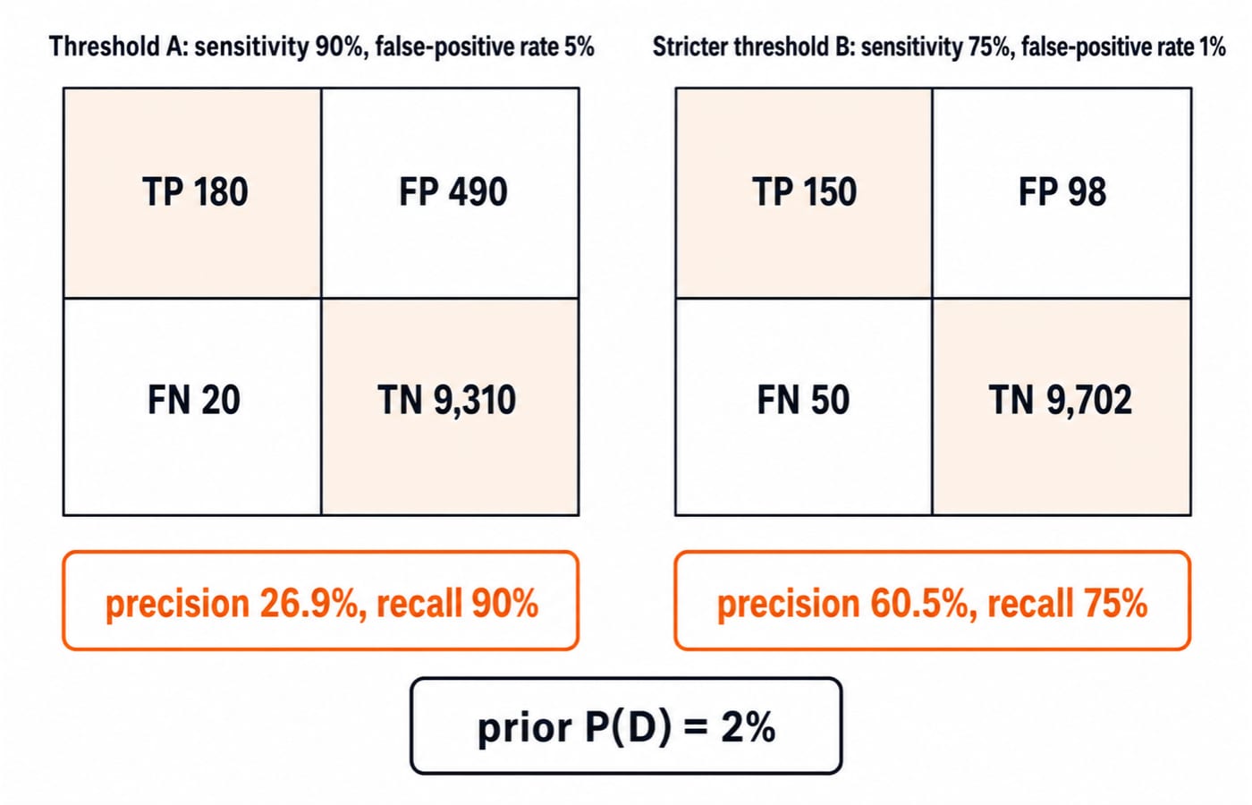
Keep the same classes, but make the threshold stricter. Point B has 75% sensitivity and a 1% false-positive rate, producing TP = 150, FP = 98, FN = 50, and TN = 9,702.
Its precision becomes 150 / (150 + 98) = 150 / 248 = 0.604838..., or about 60.5%, while recall becomes 75%. The original point A had 26.9% precision and 90% recall. The stricter threshold more than doubles precision in this teaching example but misses 30 additional actual positives.
The prior remains 2%; P(+ | D) and P(+ | not D) changed. No threshold is universally best. Choice depends on error costs and validation on the deployment population.
7. Odds form and the conditional-independence trap
At operating point A, prior odds are 0.02 / 0.98 = 1 / 49. The positive likelihood ratio is 0.90 / 0.05 = 18. Bayes' rule in odds form multiplies them:
posterior odds = (1 / 49) x 18 = 18 / 49
Convert back: 18 / (18 + 49) = 18 / 67 = 26.9%. Evidence multiplies odds.
If a second positive signal had ratio 18 and were conditionally independent of the first given each class, the odds become (18 / 49) x 18 = 324 / 49. That gives 324 / 373 = 86.86...%, about 86.9%.
Independence is essential. A reused feature, correlated measurement, or model trained on nearly identical inputs does not justify multiplication.
prior = 0.02
sensitivity = 0.90
fpr = 0.05
posterior = sensitivity * prior / (sensitivity * prior + fpr * (1 - prior))
print(f"{posterior:.4f}")  # 0.2687
For the programming foundation needed to reproduce it, try Python Course: Concepts, MCQs & Coding.
8. How ML assessments test Bayes' rule
Four common forms are:
Reverse the conditional: distinguish 90% sensitivity from 26.9% precision.
Recover the hidden denominator: rebuild
670 = 180 + 490.Change the threshold: recompute
150 / (150 + 98) = 60.5%.Inspect repeated evidence: reject the second likelihood-ratio multiplication unless conditional independence is stated.
Run a five-item trap check:
Did you swap
P(+ | D)andP(D | +)?Did you include the prior?
Did you convert specificity to false-positive rate using
1 - specificity?Did you treat an uncalibrated score as a probability?
Did you multiply correlated evidence as if it were conditionally independent?
The short version
Explain why 90% sensitivity can coexist with 26.9% precision. Rebuild all 670 predicted positives. Then explain why threshold B raises precision while recall falls. If you cannot do all three without looking back, return to the count tree before adding more formulas.
For broader model learning, use AI & ML for Placements or compare the Skill Development Courses track. Bayes' rule becomes reliable when you name the reference group, keep the prior visible, and check the formula against counts.
Keep learning
Probability Distributions for Machine Learning: Match Bernoulli, Binomial, Normal and Poisson to Data
Learn a reusable way to match binary outcomes, grouped successes, event counts and continuous residuals to a defensible probability model.
Updated 13 Nov 20266 min readML & Data Science

Probability for GATE CS
Translate the wording into events before calculating. Exact dice, Bayes and expectation examples show how to build the denominator and avoid the standard independence trap.
Updated 30 Oct 20265 min readEngineering Mathematics

Hypothesis Testing for Machine Learning: Separate Signal from Sampling Noise in Model Comparisons
Learn one complete paired-model comparison, from a 2 by 2 prediction table and exact p-value to effect size, confidence interval, test choice, and leakage checks.
Updated 17 Nov 20266 min readML & Data Science
GATE DA Machine Learning Revision Map: From Probability to Neural-Network Calculations
Connect five machine-learning note sets through four worked problems and a complete neural-network forward pass, with a focused 90-minute revision loop.
Updated 5 Nov 20265 min readML & Data Science