

Maximum Likelihood Estimation for a Bernoulli Model: Fit p by Hand
See why the Bernoulli MLE is the sample proportion. One eight-observation example builds the likelihood, solves it, and checks the result.
KnowledgeGate Team
Exam prep & CS education
Updated 12 Nov 20265 min read

A library can fit a binary model in one line, but that call hides why the fitted probability becomes one particular number. The eight recorded trials contain five successes and three failures, so the fitted Bernoulli probability is p_hat = 5/8 = 0.625.
Bernoulli maximum likelihood estimation: define the model before fitting it
One Bernoulli observation X_i takes the value 1 with probability p and 0 with probability 1-p, where 0 <= p <= 1. Its compact probability mass function is
P(X_i = x_i | p) = p^(x_i)(1-p)^(1-x_i), for x_i in {0,1}.
If x_i=1, this becomes p^1(1-p)^0=p. If x_i=0, it becomes p^0(1-p)^1=1-p.
For the product below, we model the eight outcomes as independent and identically distributed conditional on one shared, fixed p. That is an assumption about eight outcomes generated under the same process, not something proved by writing them in a list.
Before observation, P(data | p) scores possible data for a fixed p. After the data are fixed, L(p | data) is the same expression viewed as a function of candidate values of p. It does not assign probabilities to those candidates. Keeping those two readings apart is what makes the rest of this derivation easy, and the wider programming and machine-learning material sits in Coding & Skills.
Build the Bernoulli likelihood from eight observations
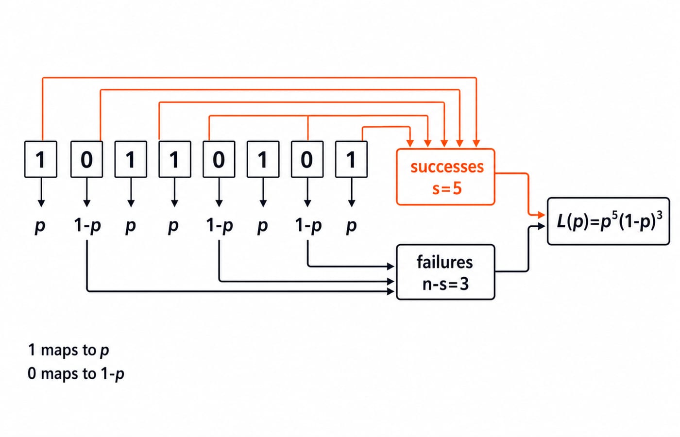
Keep the sample in its recorded order:
x = (1, 0, 1, 1, 0, 1, 0, 1), with n=8.
|
| Likelihood factor |
|---|---|---|
1 | 1 |
|
2 | 0 |
|
3 | 1 |
|
4 | 1 |
|
5 | 0 |
|
6 | 1 |
|
7 | 0 |
|
8 | 1 |
|
The count is s=sum x_i=5 successes and n-s=3 failures. Multiplying before collecting equal factors gives
L(p)=p(1-p)pp(1-p)p(1-p)p=p^5(1-p)^3.
The reusable form is
L(p)=product_i p^(x_i)(1-p)^(1-x_i)=p^s(1-p)^(n-s).
This is the likelihood of the ordered Bernoulli sample. If the only recorded datum were the count "5 successes out of 8", its binomial probability would be C(8,5)p^5(1-p)^3. Here C(8,5)=56 is constant with respect to p, so it rescales the likelihood but cannot move its maximiser. If the underlying probability rules feel shaky, refresh them first with Probability for GATE CS.
Use the log-likelihood to turn products into sums
For L(p)>0, maximising ln L(p) gives the same answer as maximising L(p) because ln is strictly increasing. Any fixed logarithm base greater than 1 has the same maximiser. For the sample,
ell(p)=ln L(p)=ln[p^5(1-p)^3]=5 ln p+3 ln(1-p), for 0<p<1.
More generally, ell(p)=s ln p+(n-s)ln(1-p). The identities ln(ab)=ln a+ln b and ln(a^b)=b ln a turn the product into a sum and bring exponents down as coefficients. This exposes the terms needed for differentiation. In larger samples, summing log probabilities also avoids repeatedly multiplying tiny numbers that can underflow in finite-precision computation. Logs do not change the estimator.
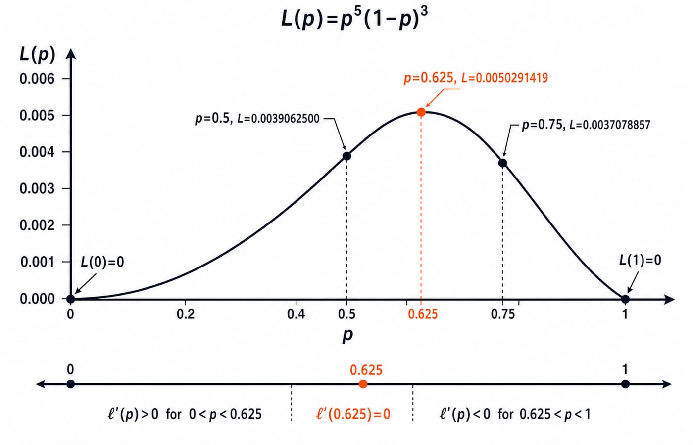
Three candidate checks are:
L(0.5)=0.5^5(0.5)^3=0.0039062500L(0.625)=0.625^5(0.375)^3=0.0050291419L(0.75)=0.75^5(0.25)^3=0.0037078857
These values suggest a peak near 0.625, but three comparisons do not prove a global maximum.
Differentiate, solve for p, and prove the maximum
Differentiate each log term, keeping the chain-rule sign visible:
ell'(p)=5/p-3/(1-p).
Set this derivative to zero and solve without skipping the algebra:
5/p=3/(1-p)
5(1-p)=3p
5-5p=3p
5=8p
Therefore, p_hat=5/8=0.625.
The general calculation fits in one chain: ell'(p)=s/p-(n-s)/(1-p)=0 implies s(1-p)=(n-s)p, hence s=np and p_hat=s/n. For binary data, that is also the sample mean:
x_bar=(1+0+1+1+0+1+0+1)/8=5/8.
Now prove that the stationary point is the maximum. The second derivative is
ell''(p)=-5/p^2-3/(1-p)^2,
which is negative for every 0<p<1. At p=0.625, it is approximately -34.1333. Also,
ell'(p)=(5-8p)/[p(1-p)].
Inside (0,1), the denominator is positive. The derivative is positive below 0.625, zero at 0.625, and negative above it. Concavity and this sign change establish the unique interior maximum.
Check the fitted model by substitution, not by faith
Substitution gives P_hat(X=1)=0.625 and P_hat(X=0)=1-0.625=0.375. They sum to 1. Under the fitted model, the estimated probability for a future outcome from the same assumed process is 0.625. This does not guarantee that the next outcome is 1, or that every future block of eight contains exactly five successes.
Candidate |
| Relative conclusion |
|---|---|---|
0.625 | 0.0050291419 | Highest of these three |
0.5 | 0.0039062500 | Lower than at 0.625 |
0.75 | 0.0037078857 | Lowest of these three |
Likelihoods compare candidates for the same fixed data. Their raw values are not probabilities that p equals those candidates.
A plain Python check verifies the estimate. No fitting library is needed:
data = [1, 0, 1, 1, 0, 1, 0, 1]
p_hat = sum(data) / len(data)
print(p_hat)
The output is 0.625.
Boundary cases and assumptions that the shortcut can hide
For (0,0,0,0), n=4, s=0, and L(p)=(1-p)^4. This decreases across [0,1], so its maximum occurs at the boundary p_hat=0. For (1,1,1,1), L(p)=p^4 increases across [0,1], so p_hat=1. The earlier log derivative assumed 0<p<1. These boundaries need separate checks because ln 0 is undefined.
If the process changes between trials, or observations depend on earlier outcomes, a single shared-p, i.i.d. Bernoulli likelihood is not justified. The arithmetic s/n still exists as a sample proportion, but calling it the MLE for that changed data-generating process would require a new likelihood.
MLE is a parameter-fitting principle used across many statistical models. The Bernoulli model is its cleanest small example because it has one parameter and binary outcomes. Approaches to AI maps the wider field that this fitting method feeds into.
Maximum likelihood traps and exam-style checks
Wrong move | Why it fails | Correct move |
|---|---|---|
Write | The counts are reversed | Five ones and three zeros give |
Treat | Likelihood is not a distribution over | Score candidate |
Lose the minus sign in | The chain rule was missed | Use |
Stop at | Stationary does not prove maximum | Check concavity, derivative sign, and boundaries |
Differentiate | It is constant in | Omit it or retain it as a constant |
Laplace smoothing gives (s+1)/(n+2)=6/10=0.6, not the MLE 5/8=0.625. Adding pseudo-counts deliberately changes the estimator, so it does not belong in an ordinary maximum likelihood calculation.
The estimator gives:
For
(1,1,0,1,0,0,1,1,1,0),n=10,s=6, sop_hat=0.6.From
L(p)=p^7(1-p)^3, infer ten trials, seven successes, andp_hat=0.7.For
(0,0,0), the boundary MLE is0.For the main sample, the computed likelihood ranking is
L(0.625) > L(0.5) > L(0.75).
For adjacent practice on how fitted models are examined, work through Artificial Neural Networks MCQs, which sit beside this derivation rather than repeating it.
Bernoulli MLE short version and the next step
Keep this five-line chain:
Encode outcomes as zero or one.
Count
ssuccesses inntrials.Write
L(p)=p^s(1-p)^(n-s).Take logs and solve
ell'(p)=0.Check concavity and boundary cases.
Here s=5 and n=8, so p_hat=0.625. Now cover up the derivation and rebuild it for (1,0,0,1,1,0). You should obtain n=6, s=3, L(p)=p^3(1-p)^3, and p_hat=0.5, then explain why the likelihood is symmetric about 0.5.
When you are ready to move from hand-fitted statistical models towards wider AI and machine-learning study, Artificial Intelligence (AI) is a broader next learning path.
Keep learning

Probability Distributions for Machine Learning: Match Bernoulli, Binomial, Normal and Poisson to Data
Learn a reusable way to match binary outcomes, grouped successes, event counts and continuous residuals to a defensible probability model.
Updated 13 Nov 20266 min readML & Data Science
Gradient Descent for Linear Regression: Derive and Run One Update by Hand
See prediction, residual, gradient and parameter update as one continuous calculation. Then verify the lower loss and test what an oversized learning rate does.
Updated 17 Nov 20265 min readML & Data Science

Recursion in C: Stack Frames, a Hand-Tracing Method and Solved GATE Questions
Trace recursive C programs without guessing. Follow factorial returns, prints on descent and unwind, Fibonacci call counts, and maximum stack depth.
Updated 30 Oct 20267 min readDSA & Algorithms

Graph Covering: Line and Vertex Covers, Independent Sets, Minimal vs Minimum, Maximal vs Maximum
Carry one six-vertex path through vertex covers, independent sets, edge covers and matchings. Exact witnesses show why local irreducibility is not global optimality.
Updated 3 Nov 20266 min readEngineering Mathematics