

Hypothesis Testing for Machine Learning: Separate Signal from Sampling Noise in Model Comparisons
Learn one complete paired-model comparison, from a 2 by 2 prediction table and exact p-value to effect size, confidence interval, test choice, and leakage checks.
KnowledgeGate Team
Exam prep & CS education
Updated 17 Nov 20266 min read

Model B scores 84.2% while Model A scores 82.0%, but that 2.2-point gap alone cannot tell you whether B is genuinely better or simply lucky on this sample. Your real problem is deciding whether a leaderboard win is a repeatable improvement or sampling noise, and whether it is big enough to act on. Preserve the paired outcomes, test the disagreement with an exact McNemar p-value, and interpret it alongside the effect size and confidence interval.
Hypothesis testing for ML starts with an estimand, not a p-value
First define Delta = P(Model B correct) - P(Model A correct) for future examples from the same deployment population. Test H0: Delta = 0 against two-sided H1: Delta != 0. Use Delta > 0 only if pre-chosen and a worse B changes the decision.
delta_hat tells you the difference observed in your sample. The p-value tells you how incompatible the data are with H0, while the effect size and interval describe plausible values of Delta. None of these gives P(H0), the probability that the null is true.
The sampling unit is one independent labelled example. Repeated users, patients, devices or time blocks require grouping, cluster-aware resampling or blocking. Build the statistical and programming foundations through Skill Development Courses.
Paired model predictions reduce to a 2 by 2 disagreement table
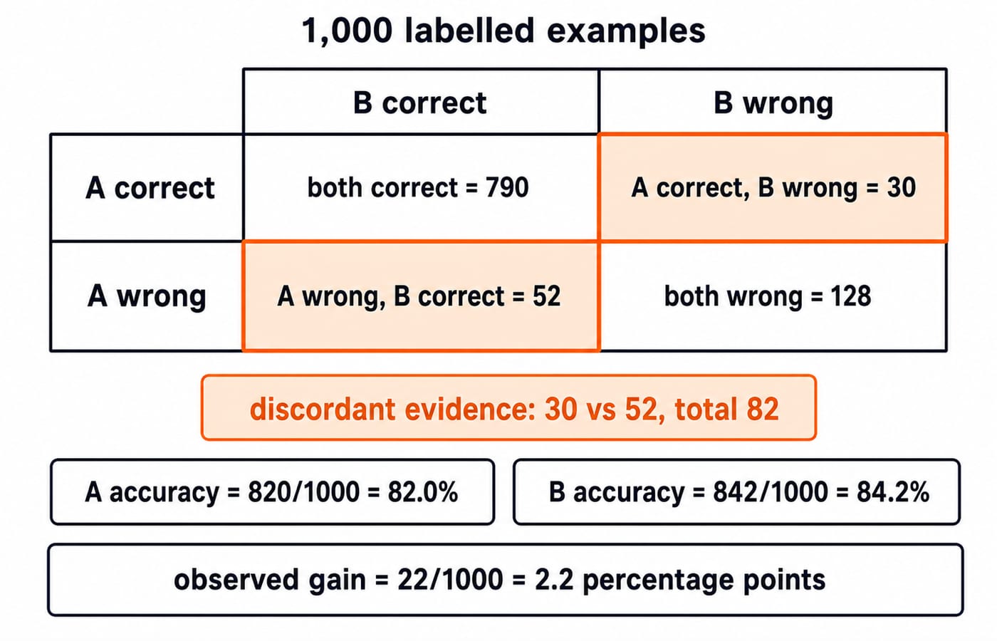
Suppose both models predict 1,000 previously untouched, independent examples.
Model B correct | Model B wrong | Row total | |
|---|---|---|---|
Model A correct | 790 | 30 | 820 |
Model A wrong | 52 | 128 | 180 |
Column total | 842 | 158 | 1,000 |
Margins give A (790 + 30)/1000 = 820/1000 = 82.0% and B (790 + 52)/1000 = 842/1000 = 84.2%. Thus delta_hat = 0.842 - 0.820 = 0.022, or 2.2 points.
An independent proportions test loses pairing. The models agree on 790 + 128 = 918 cases. The 82 disagreements are A-only b = 30 and B-only c = 52. The net is c - b = 22, not 52.
McNemar's exact test turns the 30 versus 52 split into a p-value
Under H0, each of 82 disagreements equally favours either model, so B-only wins follow X ~ Binomial(n = 82, p = 0.5). Expect 82 x 0.5 = 41; 52 is 11 higher.
The exact two-sided result is p = 2 x P(X >= 52 | X ~ Binomial(82, 0.5)) = 0.01983, rounded to 0.020. Reject H0 at pre-chosen alpha = 0.05. This supports unequal paired error behaviour, not a 98% probability that B is better.
The p-value uses the 30 versus 52 imbalance, not deployment value, data quality, calibration, fairness, latency or error cost. Review Probability for GATE CS for the binomial foundation.
Effect size and confidence interval answer the practical question
A makes 1000 - 820 = 180 errors and B makes 1000 - 842 = 158, 22 fewer per 1,000. The absolute effect is 2.2 points; relative error reduction is (180 - 158)/180 = 22/180 = 0.1222, about 12.2%. They answer different questions.
Define D: +1 for 52 B-only wins, -1 for 30 A-only wins, 0 otherwise. Its mean is (52 - 30)/1000 = 0.022. Because D is +1, -1 or 0, each of the 82 disagreements contributes 1 to the sum of squared values, so that sum is 82; dividing by n minus 1, which is 999, gives the sample variance [82 - 1000(0.022)^2]/999 = 81.516/999 = 0.08160. The standard error is sqrt(0.08160/1000) = 0.00903, and the approximate 95% interval is 0.022 +/- 1.96(0.00903) = [0.0043, 0.0397], or 0.43 to 3.97 points.
Set pre-chosen delta_min = 1 point. The estimate clears it, but the interval includes smaller gains. This supports a positive average gain, not 95% confidence that it clears the threshold or an automatic deployment verdict.
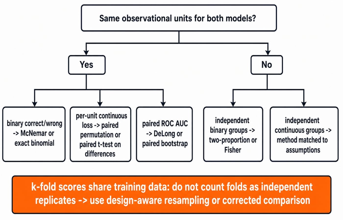
Test selection depends on pairing, outcome type and sampling design
Evaluation design | What is paired | Suitable method | Main caution |
|---|---|---|---|
Same examples, binary correct/wrong | Example predictions | McNemar or exact binomial | Independence or clustering |
Same examples, decomposable continuous loss | Example losses | Paired permutation or paired t-test on differences when reasonable | Skew and dependence |
Independently assigned user groups, binary conversions | None | Two-proportion or Fisher's exact for small counts | Assignment and exposure definitions |
Same cases, ROC AUC | Predictions, AUC is global | DeLong or paired bootstrap | Not an accuracy test |
More than two models on the same independent datasets | Dataset results | Friedman or repeated measures, then corrected comparisons | No uncorrected pairs |
K-fold scores correlate because training sets overlap. 5 folds x 10 repeats = 50 is not 50 independent observations for a naive t-test. On one dataset, use a pre-specified nested design with paired resampling or correction. Across separate datasets, pair by dataset.
Ask about pairing, outcome type and unit independence. Test names come last.
Sampling, test-set reuse and multiple comparisons can manufacture significance
Audit first: was the test set untouched during model choice? Do rows repeat users or sessions? Did preprocessing learn from it? Were thresholds selected on its labels? Does its population match deployment? A correct p-value cannot repair leakage or bias.
For 20 independent null comparisons at alpha = 0.05, at least one false positive has probability 1 - (1 - 0.05)^20 = 1 - 0.95^20 = 0.6415, about 64.2%. Tests need not be independent; repeated searches still weaken an isolated p.
Pre-register one primary metric, reserve an untouched final test set, and report planned results, including negatives. Use Holm for family-wise error or Benjamini-Hochberg for false-discovery rate. A post-hoc threshold is exploratory, not confirmatory.
ML assessments test interpretation more often than arithmetic
Typical questions ask for H0 and H1, McNemar for paired examples, a valid reading of p = 0.020, and the difference between 2.2 points and 12.2% error reduction. Never claim P(H0) = 0.020.
Swap to A-only 52 and B-only 30: p stays 0.020, but B's effect becomes -2.2 points. Set both to 41: delta_hat = 0, p is 1. Raise the useful threshold from 1 to 3 points: 2.2 fails it, while p is unchanged.
Mistake | Why it fails | Repair |
|---|---|---|
Accuracy margins only | Pairing is lost | Tabulate disagreements |
Read p as | Wrong probability | State incompatibility under |
| Non-rejection is not equivalence | Use equivalence testing |
| Size and cost are absent | Add effect, interval, threshold |
Choose one-sided after B wins | Direction came from data | Pre-specify it |
Count CV folds as independent | Training overlaps | Use design-aware methods |
Test many metrics, report smallest p | Selection inflates false positives | Correct the declared family |
Omit sampling population | Estimand is unclear | Define population and unit |
Hypothesis testing for ML: report the whole claim, then take the next step
On 1,000 previously untouched paired examples, Model B achieved 84.2% accuracy versus 82.0% for Model A. The absolute gain was 2.2 percentage points, with an approximate paired 95% confidence interval of 0.43 to 3.97 points. Among 82 disagreements, B was uniquely correct on 52 and A on 30; an exact two-sided McNemar test gave p = 0.020.
It assumes independence, representative sampling, test-set integrity and a pre-specified metric. Calculation cannot create them.
Use this six-step revision card:
Define population and unit.
State
H0,H1and minimum useful effect.Preserve pairing.
Match method to design and outcome.
Report effect, interval and p.
Audit leakage and multiplicity.
Reproduce 82, 41, 0.020, 2.2 points, 12.2%, and 0.43 to 3.97 without looking back. To take these evaluation habits further through a full applied AI course, continue with AI & ML for Placements. Then rerun it on a real paired prediction file: state its unit, lock a practical threshold, and write the result before comparing another model.
Keep learning
Probability Distributions for Machine Learning: Match Bernoulli, Binomial, Normal and Poisson to Data
Learn a reusable way to match binary outcomes, grouped successes, event counts and continuous residuals to a defensible probability model.
Updated 13 Nov 20266 min readML & Data Science

Conditional Probability for Machine Learning: Bayes' Rule with a Worked Classifier Example
Follow one hypothetical classifier from conditional probability to Bayes' posterior. Verify the answer with natural frequencies, compare precision with recall, and see exactly what a stricter threshold changes.
Updated 10 Nov 20266 min readML & Data Science

Covariance and Correlation for Machine Learning: Read Feature Relationships Correctly
Calculate covariance and Pearson correlation by hand, then see how units, influential points and nonlinear patterns change what the numbers mean.
Updated 14 Nov 20266 min readML & Data Science

GATE DA Machine Learning Revision Map: From Probability to Neural-Network Calculations
Connect five machine-learning note sets through four worked problems and a complete neural-network forward pass, with a focused 90-minute revision loop.
Updated 5 Nov 20265 min readML & Data Science