Join Operations in DBMS: Inner, Left, Right and Full Outer Joins Worked Step by Step

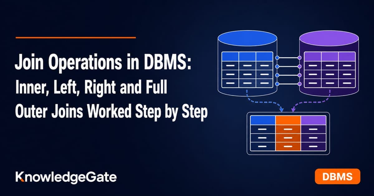
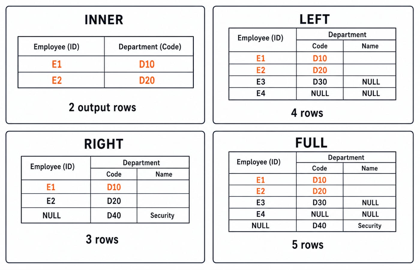
INNER, LEFT, RIGHT and FULL OUTER look like four definitions until a question asks exactly which unmatched rows survive and where NULL appears. With four Employee rows and three Department rows, the join rules produce exact outputs of 2, 4, 3 and 5 rows for INNER, LEFT, RIGHT and FULL OUTER respectively. Once you trace the matches, you should be able to predict a join result without relying on memorised Venn diagrams.

Join operations in DBMS: match rows, then decide which unmatched rows survive

A join combines rows from two relations according to a predicate. There are two separate decisions: the ON predicate decides which row pairs match, while the join type decides whether unmatched rows from the left, the right, both sides or neither side survive.

A theta join permits any comparison, an equijoin uses equality, and an inner join keeps matches only. Natural join is same-named-column shorthand, not a safer default.

In relational algebra, Employee ⋈_{Employee.DeptID = Department.DeptID} Department corresponds to an INNER JOIN. Left, right and full outer joins use ⟕, ⟖ and ⟗. As a reasoning model, four Employee rows and three Department rows give 4 × 3 = 12 possible pairs. The equality predicate in our example is true for only two pairs. A database engine need not physically build all 12 pairs.

For SELECT, filtering and subqueries, read SQL Queries and Joins in DBMS: Worked Join and GROUP BY. Place this lesson within wider revision through GATE CS Exam Preparation.

Inner join worked example: build the two source tables and keep only matches

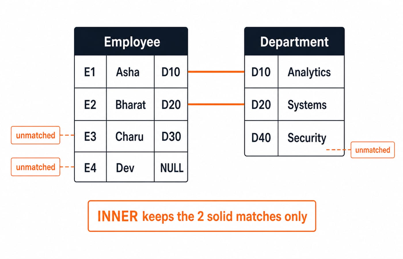
The Employee and Department tables provide the source rows for each join example.

Employee

Department

D10 matches Asha with Analytics, and D20 matches Bharat with Systems. D30, Dev's NULL, and Department's D40 are unmatched.

SELECT E.EmpID,
       E.EmpName,
       E.DeptID AS EmployeeDeptID,
       D.DeptID AS DepartmentDeptID,
       D.DeptName
FROM Employee AS E
INNER JOIN Department AS D
  ON E.DeptID = D.DeptID;

The exact result is:

The count is two, not three or four. Charu's D30 has no match, and Dev's missing key matches nothing. An inner join keeps only pairs for which ON is TRUE.

Left outer join worked example: preserve all four employee rows

Change only the keyword to LEFT OUTER JOIN; LEFT JOIN means the same. “Left” refers to Employee AS E in the query, not table size or diagram layout.

The same projection and ON E.DeptID = D.DeptID predicate produce:

The nulls have two sources. Dev's source key is already NULL. Charu has D30, but the absent Department row supplies NULL placeholders.

Start with the two inner-join rows, append each unmatched Employee once, and pad the absent Department columns with NULL. This gives four rows. An outer join does not “match nulls”; it preserves unmatched rows. Duplicate keys will show why a left join need not equal the left table's row count.

Right and full outer joins: preserve departments, then preserve both sides

A RIGHT OUTER JOIN preserves every Department row. Its output is:

Charu and Dev disappear because their non-preserved side is unmatched. Swapping table order and using a left join gives the same result where right-join syntax is avoided.

A FULL OUTER JOIN preserves unmatched rows from both sides: the two matches, Charu, Dev and Security.

The count is 2 matched pairs + 2 unmatched Employee rows + 1 unmatched Department row = 5. Standard SQL calls this FULL OUTER JOIN, but product support and emulation syntax vary.

Outer join filters and NULL: ON versus WHERE changes the answer

Start with the four-row left join and apply WHERE D.DeptName = 'Analytics'. Asha evaluates to TRUE, Bharat to FALSE, and Charu and Dev to UNKNOWN because their Department values are NULL. Since WHERE keeps only TRUE, the final result is one row: (E1, Asha, Analytics). The right-table condition makes this output behave like an inner join.

Move the condition into ON E.DeptID = D.DeptID AND D.DeptName = 'Analytics'. The left join still preserves all four employees. Asha matches Analytics; Bharat, Charu and Dev remain with NULL in the projected Department columns. ON controls which Department row can match. WHERE filters rows after the join.

Three traps follow from this logic:

• NULL = NULL is not TRUE in ordinary SQL comparison.

• Over the original left-join output, COUNT(D.DeptName) = 2 while COUNT(*) = 4.

• NATURAL JOIN can change silently if another same-named column is added to both tables.

For clear reasoning and maintainable SQL, prefer the explicit predicate ON E.DeptID = D.DeptID.

Join cardinality trap: duplicate key groups multiply rows

Suppose Orders contains (O1, C7) and (O2, C7). CustomerContact contains (C7, a@x.in) and (C7, b@x.in). Joining on CustomerID gives 2 × 2 = 4 rows for C7:

1. (O1, C7, a@x.in)

2. (O1, C7, b@x.in)

3. (O2, C7, a@x.in)

4. (O2, C7, b@x.in)

In general, if one key appears m times on the left and n times on the right, it contributes m × n inner-join rows. The relevant outer-join rule then adds unmatched preserved rows. DISTINCT may hide repeated output values, but it cannot repair a wrong predicate or a misunderstood one-to-many relationship.

To diagnose a count, verify the intended keys and uniqueness, count each key group on both sides, multiply matching group sizes, then account for unmatched preserved rows.

Join-operation questions: solve row counts and outputs systematically

Typical DBMS exercises ask you to predict an output table, count rows for a join type, identify a join from its result, translate relational algebra into SQL, or trace a right-table WHERE condition. Each form uses the same pair-counting method.

Use this five-step checklist:

1. List each distinct join-key value, including NULL.

2. Count its occurrences on the left and right.

3. For every matching non-null key, multiply m × n.

4. Append unmatched rows from the side or sides preserved by the join type.

5. Evaluate a later WHERE predicate using TRUE, FALSE and UNKNOWN.

For the main tables, D10 contributes one match and D20 contributes one. Then preservation gives INNER = 2, LEFT = 4, RIGHT = 3 and FULL = 5.

Use SQL Query MCQs: 12 Solved (SELECT, Joins, Subqueries) as the immediate practice step for query-output reasoning.

Inner and outer joins: the short version and next step

Outer joins represent the missing side with NULL. Keep two durable rules: the predicate finds matching pairs, and the join type preserves selected unmatched rows after matching. Repeated key values multiply output rows.

Without looking back, reproduce the four counts and the five full-join rows. Then move the Analytics condition between ON and WHERE and explain why the results differ. That is the minimum active-recall check before attempting MCQs.

For a structured route through DBMS, including SQL, alongside the wider GATE CS subject plan, continue with GATE Guidance by Sanchit Sir.