Image Processing in Computer Graphics: Concepts, Worked Examples, and How Exams Test It

Image processing questions look easy until a storage calculation, filter mask, or gray-level numerical appears. Students often study Computer Graphics as theory and never compute by hand. Image processing combines core concepts with standard numerical problems.

Related reading: computer graphics basics and display technologies.

What image processing is, and how it differs from computer graphics

Computer graphics synthesises images from models: a scene description, shapes, and lighting become pixels. Image processing analyses or transforms an existing image, so pixels become better pixels or new information.

Computer vision takes pixels and returns a description or decision. In short, model to image is graphics, image to image is processing, and image to description is vision. Classification questions often test this distinction.

The standard pipeline is acquisition → digitisation (sampling and quantisation) → enhancement (point and neighbourhood operations) → restoration → segmentation or analysis. The pipeline runs from representation to analysis.

Digital image representation: pixels, bit depth, and storage

A digital image is an M × N pixel matrix. A grayscale pixel stores one intensity; an RGB pixel stores three colour components. Bit depth k allows 2^k values. Therefore, 1 bit gives 2 levels, 8-bit grayscale gives 256 levels from 0 to 255, and 24-bit RGB gives 8 bits per channel.

Consider an uncompressed 1024 × 768 image. First calculate its pixel count:

1. Pixels = 1024 × 768 = 7,86,432 pixels.

2. For 8-bit grayscale, each pixel needs 8 bits = 1 byte.

3. Storage = 7,86,432 × 1 = 7,86,432 bytes.

4. Using the common exam convention 1 KB = 1024 bytes, 7,86,432 ÷ 1024 = 768 KB.

For 24-bit RGB, each pixel needs 24 bits = 3 bytes:

1. Storage = 7,86,432 × 3 = 23,59,296 bytes.

2. Using the same convention, 23,59,296 ÷ 1024 = 2,304 KB.

3. With 1 MB = 1024 KB in this convention, 2,304 ÷ 1024 = 2.25 MB.

The formula is size in bits = M × N × k, where k is total bits per pixel. For more binary storage drills, revise Number Systems and Base Conversions.

RGB is additive and suits displays. CMY and CMYK are subtractive and suit print. HSV separates brightness-like information from colour, useful when a step should change intensity without disturbing hue.

Sampling and quantisation: how a scene becomes numbers

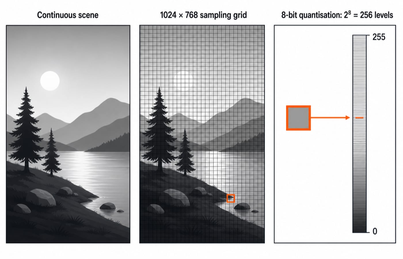
Sampling decides how many spatial points form the M × N grid. Quantisation decides how many intensity or colour levels each measurement may take.

Undersampling causes jagged or blocky detail and aliasing. Coarse quantisation causes false contouring, visible bands in a smooth gradient. Pair grid density with sampling and level count with quantisation.

An 8-bit image has 2^8 = 256 levels. Reducing it to 3 bits leaves 2^3 = 8 levels, so smooth changes become visible steps.

Point operations: negatives, thresholding, and histograms

A point operation transforms each pixel independently. For a negative, s = (L − 1) − r. With L = 256 and r = 40, s = 255 − 40 = 215.

Thresholding compares input with a fixed value. At T = 128, r = 40 becomes 0 (black) and r = 200 becomes 255 (white), producing a binary image.

A brightness shift may use s = r + 50, but 8-bit values end at 255. For r = 230, 230 + 50 = 280, clipped to 255.

A histogram counts pixels at each gray level. A dark image is bunched left; a low-contrast image has a narrow histogram. Histogram equalisation uses a cumulative-distribution table to redistribute occupied levels and improve contrast.

Neighbourhood operations: mean and median filters

In a neighbourhood operation, the output depends on nearby pixels, commonly a 3 × 3 window. Applying its mask or rule is a central numerical.

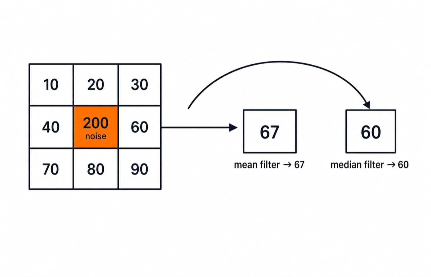
Take this neighbourhood, where the centre value 200 is a salt-noise spike:

For a mean filter, add all nine values:

10 + 20 + 30 + 40 + 200 + 60 + 70 + 80 + 90 = 600

Mean = 600 ÷ 9 = 66.67, which rounds to 67. The new centre value is 67.

For a median filter, sort the values:

10, 20, 30, 40, 60, 70, 80, 90, 200

With nine values, the median is the fifth, 60. The outlier pulls the mean to 67, while the median ignores its magnitude and returns 60. That is why median filtering is the standard choice for salt-and-pepper noise. "Mean removes impulse noise best" is a designed-to-fail option.

Edge detection: gradients and a worked Sobel operator

An edge is where intensity changes sharply. Gradient masks estimate that change. The Sobel Gx kernel is:

-1  0  1
-2  0  2
-1  0  1

Gy is its transpose-style vertical counterpart. Apply Gx to a patch that changes from 50 to 150 across each row:

50  50  150
50  50  150
50  50  150

Multiply matching entries and add them:

Gx = (−1)(50) + (0)(50) + (1)(150) + (−2)(50) + (0)(50) + (2)(150) + (−1)(50) + (0)(50) + (1)(150)

= (−50 + 150) + (−100 + 300) + (−50 + 150)

= 100 + 200 + 100 = 400

For Gy, identical rows receive opposite vertical weights, so they cancel and Gy = 0. Large |Gx| with zero Gy marks a strong vertical edge. Gx names the change direction; the edge itself runs vertically.

Prewitt uses the same idea with weights of 1 instead of Sobel's central 2. The Laplacian is a second derivative, responds in all directions, and is more noise-sensitive.

Common traps and how the topic is tested

Watch for these nearly correct ideas:

• Sampling and quantisation are interchangeable. They are not. Sampling controls grid density and is tied to aliasing; quantisation controls level count and is tied to false contouring.

• The storage answer can stay in bits. Check the unit and remember RGB's three channels. Missing ×3 turns 2.25 MB into the 768 KB grayscale result.

• A mean filter is always smoother, so it must beat a median filter. The worked window disproves this for impulse noise: the mean gives 67, while the median gives 60.

• Gx detects a horizontal edge. Gx measures change along x, so it responds strongly to an edge that runs vertically.

• Computer graphics and image processing are the same pipeline. Graphics starts from a model; processing starts from an image.

Expect concept classifications, compact numericals like those above, and interview one-liners on median filtering or HSV. Pattern practice through the GATE Test Series exposes unit and direction traps. Use UGC NET Computer Science High-Yield Topics for a wider revision view, then place this compact block against your core-subject workload.

Image processing revision

• Image storage is M × N × k bits.

• Sampling sets spatial grid density; quantisation sets the number of levels.

• Point operations act on one pixel at a time.

• For the noise window above, median gives 60 while mean gives 67.

• For the vertical edge patch, Sobel Gx gives 400 and Gy gives 0.

Redo the storage, filtering, and Sobel numericals until you can complete them without looking at the steps. For structured coverage across CS subjects, continue with GATE Guidance by Sanchit Sir. Use Computer Graphics, Multimedia & Mobile Computing lessons to continue into adjacent display and graphics topics.