3-D Object Representation, Geometric Transformations and Viewing: Computer Graphics Guide with Worked Examples

Computer-graphics questions become difficult when a familiar object must move through 4x4 matrices, a camera, a projection and a viewport. Choosing the representation sets the geometry; matrix order sets the coordinates. With column vectors, the rightmost matrix acts first, and each worked point can be checked stage by stage.

The 3-D graphics pipeline in five stages

Think of the unit as one assembly line:

1. Object representation stores polygons, analytic surfaces or curves.

2. Modelling transformations place, rotate and resize the object.

3. Viewing transformation expresses the world relative to a camera.

4. Projection converts 3-D camera coordinates to a 2-D plane.

5. Window-to-viewport mapping places the result on a display area.

Homogeneous coordinates write a point as (x, y, z, 1). The extra coordinate makes translation a matrix multiplication, allowing every stage to be composed into one 4x4 matrix.

Representing 3-D objects: meshes, quadrics, splines and Bezier curves

A polygon mesh stores vertices, edges and polygon faces in linked tables. This boundary representation suits hardware rendering because it breaks a surface into simple polygons.

Quadric surfaces are exact analytic shapes described by second-degree equations. Spheres, ellipsoids and cylinders belong here. Splines describe smooth freeform curves or surfaces, so they are useful in design systems where shape control matters.

A quadratic Bezier curve with control points P0, P1 and P2 is

B(t) = (1-t)^2 P0 + 2t(1-t) P1 + t^2 P2.

Take P0 = (0,0), P1 = (2,4), P2 = (4,0) and t = 0.5. Then (1-t)^2 = 0.25, 2t(1-t) = 0.5, and t^2 = 0.25:

B(0.5) = 0.25(0,0) + 0.5(2,4) + 0.25(4,0)

B(0.5) = (0,0) + (1,2) + (1,0) = (2,2).

The curve passes through P0 and P2, stays inside the control-point convex hull, and has endpoint tangents along P0P1 and P1P2. It does not pass through P1. With n+1 control points, a Bezier has degree n, and one moved point affects the whole curve. A B-spline can keep a fixed degree and gives local control.

Geometric transformations: five core 4x4 matrices

Using column vectors, the core matrices are:

T(tx,ty,tz) = [1 0 0 tx]    S(sx,sy,sz) = [sx 0  0  0]
               [0 1 0 ty]                   [0  sy 0  0]
               [0 0 1 tz]                   [0  0  sz 0]
               [0 0 0 1 ]                   [0  0  0  1]

Rx(theta) = [1  0           0          0]
            [0  cos(theta) -sin(theta) 0]
            [0  sin(theta)  cos(theta) 0]
            [0  0           0          1]

Ry(theta) = [ cos(theta) 0 sin(theta) 0]
            [ 0          1 0          0]
            [-sin(theta) 0 cos(theta) 0]
            [ 0          0 0          1]

Rz(theta) = [cos(theta) -sin(theta) 0 0]
            [sin(theta)  cos(theta) 0 0]
            [0           0          1 0]
            [0           0          0 1]

The five matrices cover translation, scaling and rotation about each principal axis. Reflection is scaling with one or more factors set to -1. A shear uses an off-diagonal term, such as x' = x + shxy*y.

Use 2-D Transformations and Viewing in Computer Graphics for the canonical 3x3 arbitrary-pivot rotation and 2-D viewport arithmetic. The 4x4 forms add a z coordinate, 3-D model placement and fixed-point scaling.

To transform about a fixed point F, move F to the origin, transform, then move it back. For scaling, M = T(F) S T(-F). Scale P = (2,1,3) by (2,2,2) about F = (1,1,1):

P - F = (1,0,2), scaling gives (2,0,4), and adding F gives P' = (3,1,5).

Worked composite transformation: why order matters

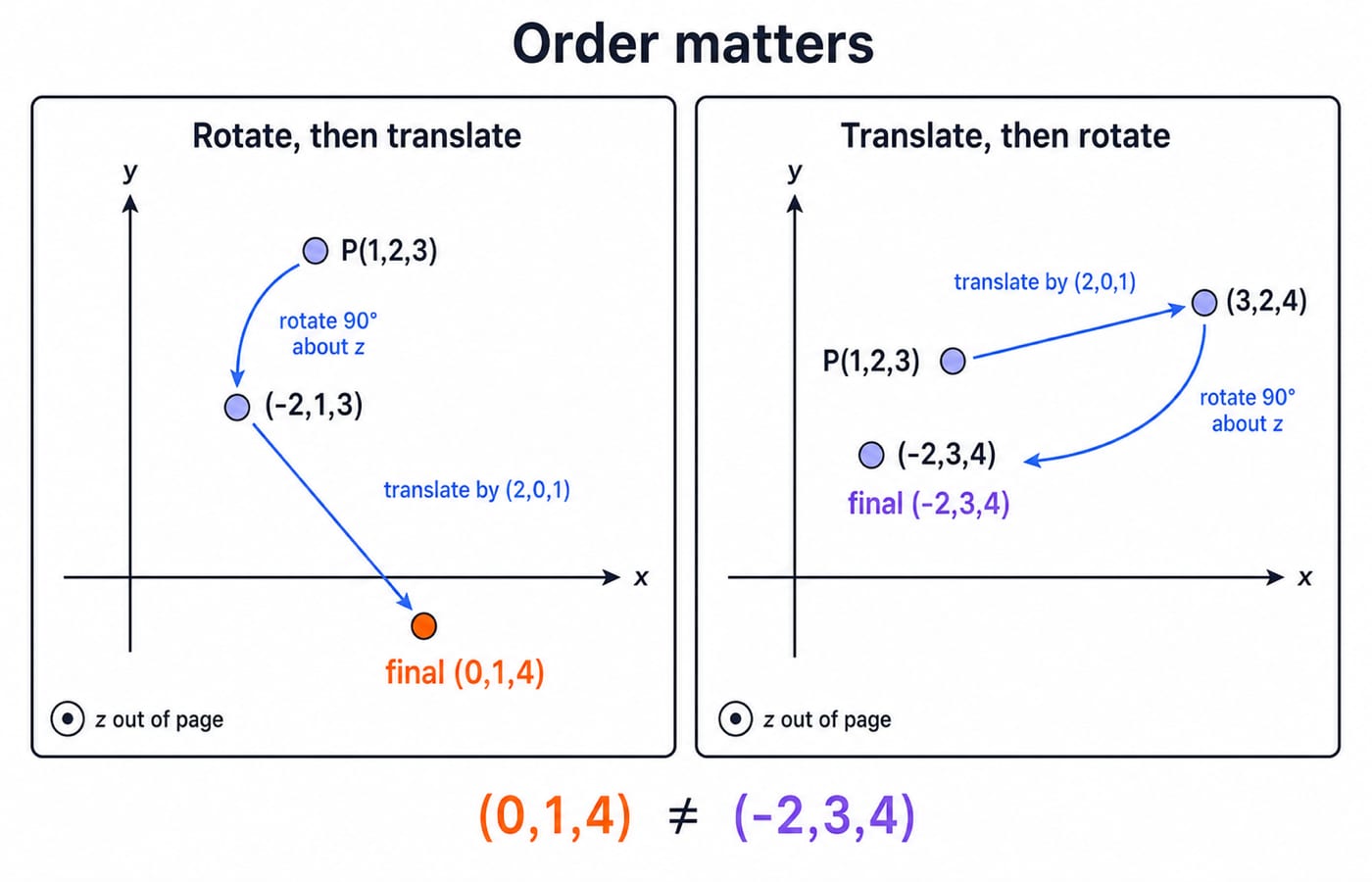
Let P = (1,2,3). Apply a 90 degree rotation about the z-axis and a translation T(2,0,1). For 90 degrees, cos 90 = 0 and sin 90 = 1.

Case 1: rotate, then translate

x' = 1(0) - 2(1) = -2

y' = 1(1) + 2(0) = 1

The rotation produces (-2,1,3). Translation then gives (-2+2, 1+0, 3+1) = (0,1,4).

Case 2: translate, then rotate

Translation first gives (1+2, 2+0, 3+1) = (3,2,4). Rotation then gives x' = -2, y' = 3, so the result is (-2,3,4).

The final points (0,1,4) and (-2,3,4) differ. Matrix multiplication does not commute. In the column-vector convention, the matrix written nearest the point acts first: P' = T R P applies R before T.

3-D viewing: from world coordinates to the screen

Viewing converts world coordinates to camera coordinates using a view reference point, view-plane normal and view-up vector. Projection places them on a view plane. Normalisation and device mapping then produce screen coordinates.

In parallel projection, projectors remain parallel. They are perpendicular to the view plane in orthographic projection and angled in oblique projection. This preserves relative proportions and suits engineering drawings. In perspective projection, projectors converge at a centre of projection, producing foreshortening and vanishing points. Perspective is not uniform scaling because apparent size depends on depth.

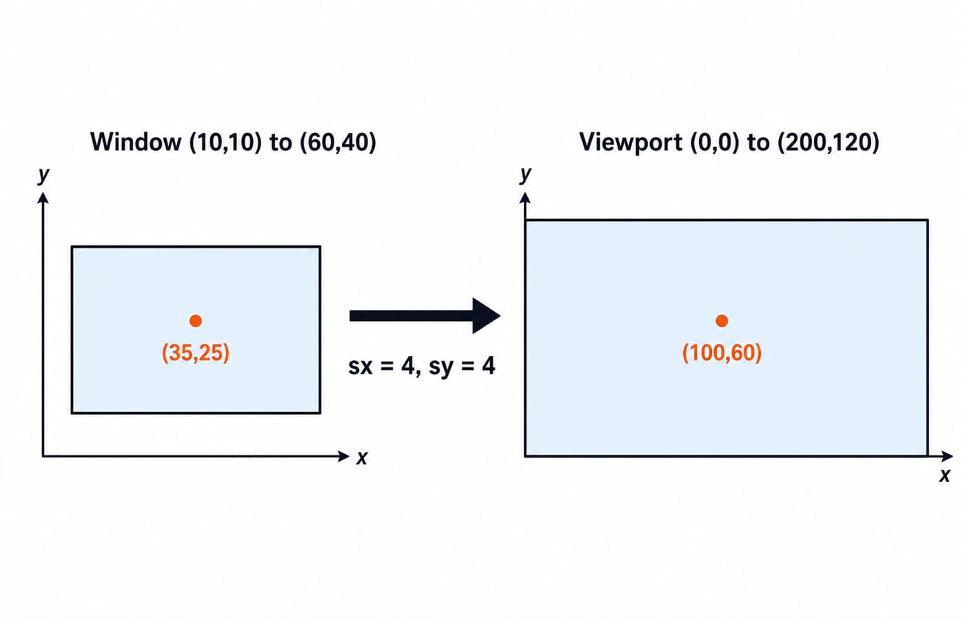
Now map a window with xw in [10,60], yw in [10,40] to a viewport with xv in [0,200], yv in [0,120].

sx = (200-0)/(60-10) = 200/50 = 4

sy = (120-0)/(40-10) = 120/30 = 4

For (xw,yw) = (35,25), use xv = xv_min + (xw-xw_min)sx and the corresponding y formula:

xv = 0 + (35-10)4 = 100, and yv = 0 + (25-10)4 = 60.

The mapped point is (100,60).

Traps that cost marks in this unit

• Dropping the fixed-point sandwich: S alone scales about the origin. Use T(F) S T(-F), then check that the example reaches (3,1,5).

• Reading a composite backwards: row-vector and column-vector conventions reverse the written order. State your convention and test the matrix on one point.

• Forcing a Bezier curve through every control point: it interpolates the endpoints, while middle points control shape and tangents. Here B(0.5) = (2,2), not P1 = (2,4).

• Mixing projection types: classify parallel projections by projector direction, and perspective by projectors converging at a centre.

• Losing rotation signs: memorise Rz, then derive Rx and Ry by the cyclic replacement x -> y -> z -> x.

Where this unit is tested

The Computer Graphics portion of UGC NET Computer Science includes 3-D object representation, geometric transformations and viewing. Use the official NTA UGC NET site to confirm the authoritative syllabus and current information bulletin, without relying on old paper-pattern details. The UGC NET Computer Science high-yield topics guide can help you place this unit in a wider revision plan.

Computer Graphics is not part of the current GATE CS core syllabus. It is relevant to UGC NET, PGT and TGT computer science recruitment papers, university examinations, and graphics or game-development interviews. For a GATE route, prioritise the listed core syllabus before treating graphics as interview-side extension.

Typical questions ask you to evaluate a Bezier point, find coordinates after a composite transformation, select the correct matrix, classify a projection, or map a point to a viewport. An interview may ask why homogeneous coordinates are useful or why transformation order changes the result.

The short version and your next step

Choose meshes for renderable boundaries, quadrics for exact analytic shapes, and splines for smooth design control. Use homogeneous 4x4 matrices and write down your vector convention before composing them. Remember the order check: P(1,2,3) became (0,1,4) one way and (-2,3,4) the other. Finish by tracing the viewing, projection and viewport stages in sequence.

For structured coverage of the complete unit, continue with NTA-UGC-NET Paper - 2. For end-to-end preparation, explore UGC NET Computer Science and Applications by Sanchit Sir, or compare the test-series routes on the UGC NET Preparation Courses & Test Series page.