

Descriptive Statistics for ML: Mean, Variance, IQR and Robust Summaries
Work through one seven-value feature to see how ordinary and robust summaries react to a long right tail. Then turn the results into careful preprocessing choices.
KnowledgeGate Team
Exam prep & CS education
Updated 11 Nov 20266 min read

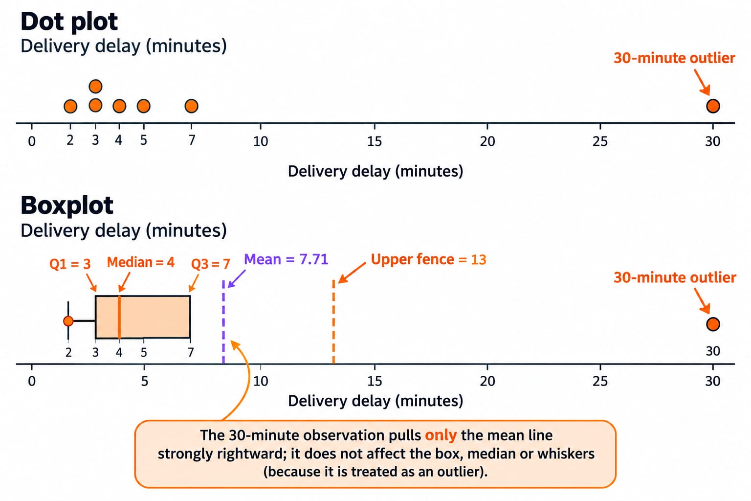
A single average can make a feature look ordinary even when most observations cluster tightly and one value stretches the scale. Consider delivery delays [2, 3, 3, 4, 5, 7, 30] minutes: six are within 7 minutes, but one is 30. Computing centre, ordinary spread and robust spread by hand helps decide what to inspect before an ML transformation or model. The 30-minute observation stretches the mean and standard deviation while leaving the median unchanged, so mean and standard deviation are insufficient here.
Descriptive statistics are a feature audit, not one magic number
Descriptive statistics compress observed data. Centre covers mean, median and mode; spread covers range, variance and standard deviation; robust summaries include median, quartiles, IQR and median absolute deviation (MAD). Compression hides detail, so also report units, count and shape. The Skills category offers broader applied technical learning.
Observation | Delay (minutes) |
|---|---|
D1 | 2 |
D2 | 3 |
D3 | 3 |
D4 | 4 |
D5 | 5 |
D6 | 7 |
D7 | 30 |
Here, n = 7, minimum 2, maximum 30, and six values lie from 2 to 7. The value 30 is unusual here, but summaries cannot blame data, traffic, weather or another delivery class.
Mean, median and mode answer different centre questions
Mean numerator:
2 + 3 + 3 + 4 + 5 + 7 + 30 = 54
Thus mean = 54 / 7 = 7.714285..., or 7.71 minutes. It is the balance-point delay, not necessarily a typical delivery's experience.
The sorted list's median position is (7 + 1) / 2 = 4, so median = 4 minutes. Mode is 3 minutes because it appears twice. Here it is just a repeated observed value, not a measure that always suits continuous data.
Mean, median and mode are 7.71, 4 and 3 minutes. The 30-minute value lifts the mean without changing the middle position. With the visible long right tail, mean > median is consistent with right skew here, but the inequality alone never proves skew.
Range, variance and standard deviation quantify ordinary spread
Range is 30 - 2 = 28 minutes. It ignores the five values between its endpoints and remains measured in minutes.
For this batch, use population variance with mean 54/7 and denominator n = 7:
Value | Squared deviation from |
|---|---|
2 | 32.6531 |
3 | 22.2245 |
3 | 22.2245 |
4 | 13.7959 |
5 | 7.3673 |
7 | 0.5102 |
30 | 496.6531 |
They sum to 595.4286. Population variance is 595.4286 / 7 = 85.0612 minutes squared; population standard deviation is sqrt(85.0612) = 9.2229 minutes. Only SD returns to the original unit.
If these records are a sample estimating a wider population, divide by n - 1 = 6: sample variance 99.2381 minutes squared, sample SD 9.9618 minutes. State the denominator and convention.
Median, IQR and MAD stay stable when the tail stretches
Using Tukey's median-of-halves convention, exclude the overall median because n is odd. Lower half [2, 3, 3] gives Q1 = 3; upper half [5, 7, 30] gives Q3 = 7; IQR = 7 - 3 = 4 minutes. Software interpolation can differ on small datasets, so record the method.
The 1.5 x IQR fences are 3 - 1.5(4) = -3 and 7 + 1.5(4) = 13. Since 30 > 13, investigate it. A fence is diagnostic, not proof of error or a deletion command.
Absolute deviations from median 4 are [2, 1, 1, 0, 1, 3, 26]; sorted, [0, 1, 1, 1, 2, 3, 26]. Their median gives raw MAD = 1 minute. Some workflows rescale MAD, so label any scaled convention.
One sensitivity check reveals which summaries are robust
Change only the tail value from 30 to 60:
Summary | Original tail | Changed tail |
|---|---|---|
Mean | 7.71 |
|
Median | 4 | 4 |
Range | 28 |
|
IQR | 4 | 4 |
Raw MAD | 1 | 1 |
Mean rises by 4.29 minutes and range by 30 minutes; median, IQR and raw MAD stay fixed. Robustness means limited sensitivity to extremes, not superiority. For symmetric, clean data, mean and SD retain every observation and may fit better.
Report: n = 7; median = 4 minutes; IQR = 4 minutes; mean = 7.71 minutes; SD = 9.22 minutes; one value, 30, lies above the 13-minute Tukey fence. Seven records cannot establish a stable population shape or choose a model.
Turn the summaries into a defensible ML preprocessing decision
Investigate before deleting. Check the record's units, collection logic, missing-value encoding, duplicate status and context. Correct a genuine entry error with an audit trail; retain a valid rare event. Never remove it just to reduce the mean.
Standard scaling with mean 7.7143 and population SD 9.2229 maps 30 to (30 - 7.7143) / 9.2229 = 2.42. Robust scaling with median 4 and IQR 4 maps values to [-0.50, -0.25, -0.25, 0, 0.25, 0.75, 6.50]. It stops the tail defining centre and scale, but neither erases it nor guarantees a better model.
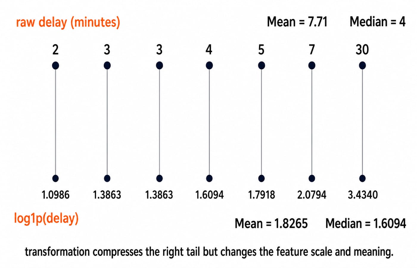
One candidate, log1p(x), maps these non-negative values to [1.0986, 1.3863, 1.3863, 1.6094, 1.7918, 2.0794, 3.4340], with mean 1.8265 and median 1.6094. It changes interpretation, so justify it through feature meaning and validation. Fit transformations on training data, then apply them unchanged to validation and test data.
Dependency-free Python keeps the conventions explicit:
from math import sqrt

x = sorted([2, 3, 3, 4, 5, 7, 30])
n = len(x)
mean = sum(x) / n
variance = sum((value - mean) ** 2 for value in x) / n
sd = sqrt(variance)
median = x[n // 2]
lower = x[:n // 2]
upper = x[n // 2 + 1:]
q1 = lower[len(lower) // 2]
q3 = upper[len(upper) // 2]
iqr = q3 - q1
absolute_deviations = sorted(abs(value - median) for value in x)
mad = absolute_deviations[n // 2]

print(f"mean {mean:.4f}, variance {variance:.4f}, sd {sd:.4f}")
print(f"median {median:.4f}, Q1 {q1:.4f}, Q3 {q3:.4f}")
print(f"IQR {iqr:.4f}, MAD {mad:.4f}")
Output is mean 7.7143, variance 85.0612, sd 9.2229; median 4.0000, Q1 3.0000, Q3 7.0000; IQR 4.0000, MAD 1.0000. The Python course builds the programming foundation this snippet assumes.
Assessment and interview-style questions test calculation plus judgement
Stable question forms include computing a missing summary, finding the measure most changed by an extreme, distinguishing variance from SD units, choosing ordinary or robust summaries, detecting denominator mismatch, and explaining why a fence does not prove error.
Four rapid checks:
If
30becomes60, what happens? Mean becomes12; median remains4.Is
30flagged by Tukey's rule? Yes. The upper fence is13.What are the two variances? Population
85.0612; sample99.2381.What is robust-scaled
30?(30 - 4) / 4 = 6.50.
Trap | What goes wrong | Repair |
|---|---|---|
Call | Hides median | Report both |
Write SD as | Confuses variance and SD | Use SD |
Compare variance with raw data | Units differ | Label squared minutes |
Use | Denominator and label conflict | Use |
Accept a software quartile silently | Convention is unknown | Record Tukey's method |
Delete | A flag becomes a verdict | Investigate context |
Scale before splitting | Validation information leaks | Fit on training only |
Probability for GATE CS moves from describing observations to reasoning about uncertainty.
Descriptive statistics for ML: the short version and next step
Inspect units and raw values.
Report
n.Compute more than one centre.
Pair range with variance or SD.
Add median, IQR and MAD when tails matter.
Investigate unusual records before transforming.
Headline: mean 7.71, median 4, population SD 9.22, IQR 4, raw MAD 1. Without looking back, reproduce sum 54, fourth-position median 4, upper fence 13 and raw MAD 1, then explain why 30 changes mean more than median.
For the wider domain, work through the Artificial Intelligence (AI) course. For another mathematical pillar of ML, study Linear Algebra for GATE CS. Next, run this template on a real feature, record the quartile convention, and validate any transformation.
Keep learning

Data and Statistics Basics MCQs and Short Answers: Mean, Data Literacy and AI
Practise a mixed set on data and statistics basics. Check six MCQs with option-by-option reasoning, then build five short answers with definitions, purpose and worked examples.
Updated 7 Nov 20268 min readML & Data Science
Range, Mean Deviation, Variance and Standard Deviation: 12 Questions with Solutions
Practise 12 questions on dispersion, from finding a range to recovering a missing number. Each solution shows the calculation and the trap to avoid.
Updated 2 Nov 20267 min readDiscrete Mathematics MCQs

JavaScript Destructuring and Spread: Syntax, Rest Patterns, and Worked Examples
Learn how JavaScript destructuring binds values, how rest collects them, and how spread expands them. Follow one object through runnable examples and common traps.
Updated 12 Sep 20265 min readWeb Development
Statistics for Competitive Exams: Concepts, Shortcuts and Solved Examples
Learn how to choose the right statistic, turn data into a useful table, calculate efficiently, and catch errors through solved examples and sanity checks.
Updated 6 Nov 20266 min readAptitude & Reasoning