Greedy algorithms: strategy, exchange arguments and classic problems
Greedy algorithms explained: greedy-choice property, activity selection, a traced Huffman tree, fractional knapsack, and where greedy fails on 0/1 knapsack.
KnowledgeGate Team
Exam prep & CS education
Updated 29 Jul 20266 min read
A greedy algorithm builds a solution one step at a time, always taking the choice that looks best right now and never reconsidering it. When it works, it is the simplest and fastest strategy there is. The danger is that a locally best choice is not always globally best, so the real skill is knowing when greedy is provably correct and when it quietly gives a wrong answer. Two properties decide it. Where both hold, as in activity selection, Huffman coding and fractional knapsack, the greedy answer is provably optimal; where one of them fails, as in 0/1 knapsack, greedy can be beaten by a wide margin.
The greedy-choice property and optimal substructure
A problem yields to a greedy algorithm when it has both of these:
Greedy-choice property. A globally optimal solution can be reached by making a locally optimal choice at each step. You never have to look ahead or undo a decision.
Optimal substructure. After the greedy choice, what remains is a smaller instance of the same problem, and an optimal solution to the whole contains optimal solutions to that subproblem.
Optimal substructure is shared with dynamic programming. The extra ingredient, the greedy-choice property, is what lets greedy commit immediately instead of exploring alternatives the way DP does. Proving that a greedy choice is safe is usually done with an exchange argument: take any optimal solution, show you can swap in the greedy choice without making it worse, and conclude the greedy choice is present in some optimal solution.
Activity selection: the cleanest greedy proof
You are given n activities, each with a start and finish time, and a single resource that can run one activity at a time. Select the maximum number of mutually compatible activities.
The greedy rule: always pick the activity that finishes earliest among those still compatible with what you have chosen. Sort by finish time, take the first, then repeatedly take the next activity whose start is at or after the last chosen finish.
Consider activities with (start, finish) pairs (1,4), (3,5), (0,6), (5,7), (3,9), (5,9), (6,10), (8,11), (8,12), (2,14), (12,16). Sorted by finish time, greedy picks (1,4), then (5,7), then (8,11), then (12,16): four activities.
The exchange argument shows that four is optimal rather than lucky. Let g be the earliest-finishing activity overall and take any optimal selection S. If S already contains g, there is nothing to prove. Otherwise let a be the earliest-finishing activity in S. Because S is compatible, every other activity in S starts at or after a finishes, and g finishes no later than a, so swapping a out for g leaves the set compatible and exactly the same size. Some optimal selection therefore contains g. Discard the activities that clash with g and the same argument applies to the smaller instance that remains, which is optimal substructure doing its job.
The rival rules really do fail. Earliest start takes (0,6) first, which blocks both (1,4) and (5,7) and caps that run at three activities. Shortest duration fails on a list as small as (0,5), (4,6), (5,10): the two-unit activity (4,6) is the shortest and clashes with both of the others, so it scores one where (0,5) plus (5,10) scores two. Spotting that gap is exactly what examiners probe.
Huffman coding: a traced tree
Huffman coding builds an optimal prefix-free binary code, giving shorter bit strings to more frequent symbols. The greedy rule: repeatedly merge the two lowest-frequency nodes into a new node whose frequency is their sum, until one tree remains.
Take six symbols with frequencies a:5, b:9, c:12, d:13, e:16, f:45. Build the tree by always combining the two smallest available frequencies:
Merge a:5 and b:9 into a node of 14.
Merge c:12 and d:13 into a node of 25.
Merge the 14-node and e:16 into a node of 30.
Merge the 25-node and the 30-node into a node of 55.
Merge f:45 and the 55-node into the root of 100.
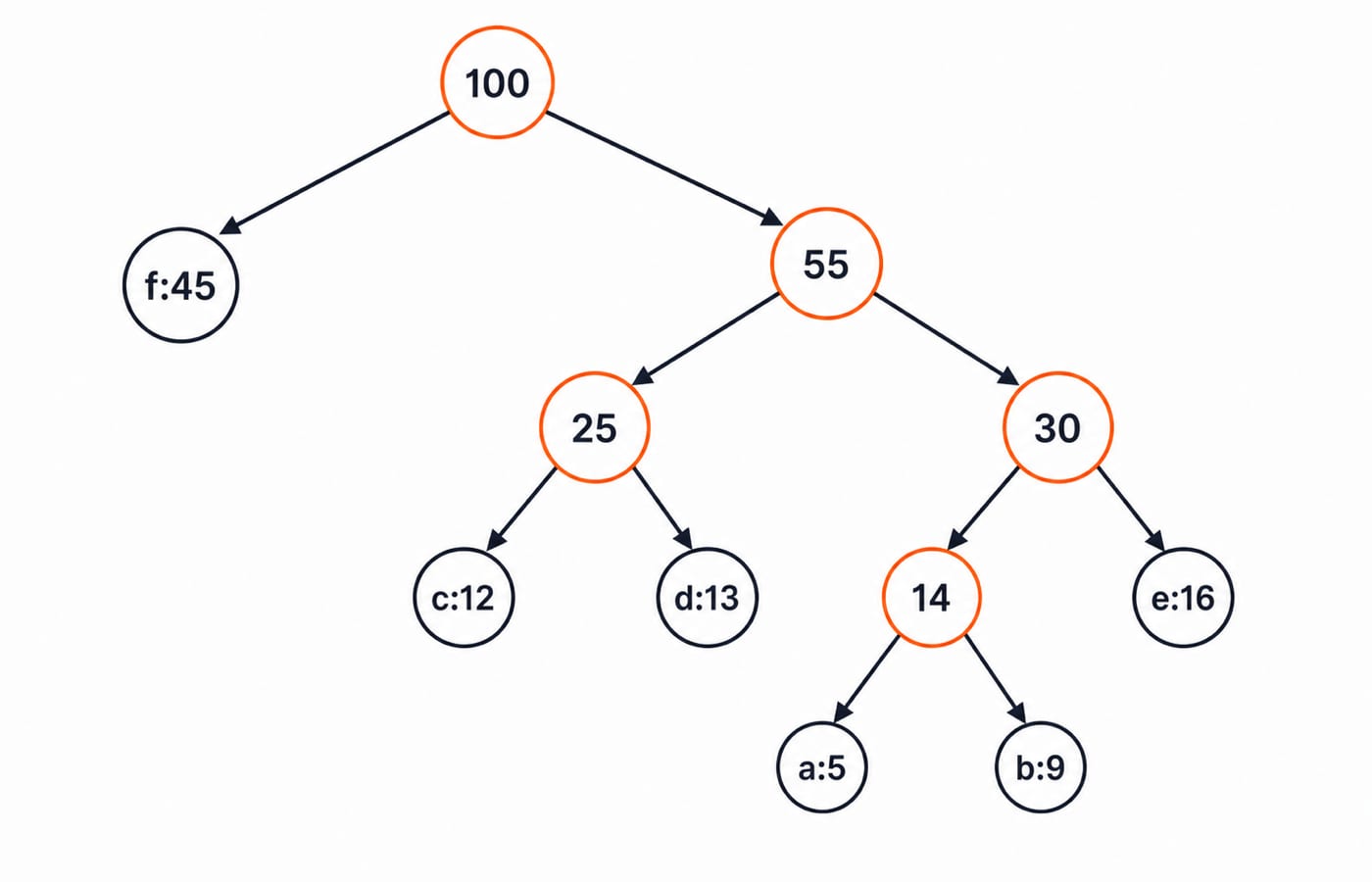
Reading left branches as 0 and right as 1, the frequent symbol f gets a 1-bit code while rare a and b get 4-bit codes. Because no code is a prefix of another, the stream decodes unambiguously. The greedy merge is optimal by an exchange argument on the two deepest, least-frequent leaves.
Fractional knapsack: greedy wins here
In the fractional knapsack you have items with weights and values and a bag of capacity W, and you may take fractions of items. Maximise the value carried. The greedy rule: take items in decreasing order of value-to-weight ratio, filling the bag and taking a fraction of the last item that fits.
With items (value, weight) of (60, 10), (100, 20), (120, 30) and capacity 50, the ratios are 6, 5, and 4 per unit weight. Greedy takes item 1 whole (10 units, value 60), item 2 whole (20 units, value 100), then 20 of the remaining 30 units of item 3 (two-thirds of value 120 = 80), for a total value of 240 in exactly 50 units of capacity. The ratio order is provably optimal because any unit of capacity is best spent on the densest value available.
Where greedy fails: 0/1 knapsack
Change one rule and greedy collapses. In the 0/1 knapsack each item must be taken whole or left behind, no fractions. Now the ratio-greedy strategy can be wrong. Take items (value, weight) of (60, 10), (100, 20), (120, 30) with capacity 50. Ratio order takes items 1 and 2 for value 160 and weight 30, leaving 20 capacity that item 3 cannot use whole. But taking items 2 and 3 gives value 220 in weight 50, which is better. Greedy misses it because it cannot reconsider the earlier commitment.
The 0/1 knapsack needs dynamic programming, which keeps every partial trade-off in a table instead of committing early. This pairing is the textbook illustration of the boundary between the two strategies, and our dynamic programming explained deep dive works the full 0/1 knapsack DP table that greedy cannot solve.
Greedy in graphs
Two of the most important graph algorithms are greedy. Prim's and Kruskal's minimum-spanning-tree algorithms both grow a tree by repeatedly adding the cheapest safe edge, and Dijkstra's shortest-path algorithm greedily finalises the nearest unvisited vertex at each step. Their correctness rests on the same exchange-argument logic, applied to a cut or a shortest-path prefix. For the traversal and shortest-path machinery underneath, our graph algorithms: BFS, DFS and shortest paths deep dive builds it from scratch.
How greedy algorithms are tested
GATE CS asks two kinds of question. The first is a worked instance: trace activity selection, build a Huffman tree and read off code lengths or the total encoded bits, or run fractional knapsack. The second is conceptual: given a problem, decide whether greedy is optimal, or spot the counterexample where it is not, with 0/1 knapsack the standard trap. Prim, Kruskal, and Dijkstra as greedy methods appear throughout the algorithms and graph sections. KnowledgeGate's question bank carries over 100 questions on greedy algorithms and over 90 on minimum spanning trees, so the practice on Huffman traces and MST cuts is substantial.
Placement interviews ask you to justify why a greedy choice is safe, code Huffman or interval scheduling, and articulate when you would switch to DP. The exchange-argument instinct is what they are testing.
The short version
Greedy commits to the locally best choice and never looks back, and it is correct exactly when the problem has the greedy-choice property on top of optimal substructure. Activity selection, Huffman coding, and fractional knapsack are the three you must be able to trace by hand; 0/1 knapsack is the one you must recognise as needing dynamic programming instead.
Build one Huffman tree and one activity-selection trace, then contrast fractional with 0/1 knapsack until the boundary is instinctive.
Work the full topic with solved problems in the Algorithms learn module.
For a GATE-depth treatment that teaches greedy alongside DP and graphs, GATE Guidance by Sanchit Sir is built for it, and placement aspirants can start from the CS Fundamentals category.
Learn to prove one greedy choice safe with an exchange argument, and you will know instantly which problems yield to greedy and which do not.
Keep learning
Tree Data Structure: Types, Traversals and a Worked BST Example
Build one nine-node binary search tree, classify its shape, trace four traversals, and work through insertion, search, deletion and complexity checks.
Updated 21 Oct 20266 min readDSA & Algorithms
Graphs in Data Structures: Complete Guide with BFS, DFS and Dijkstra Worked Examples
Learn graph terminology, representations and algorithm selection by tracing one unweighted graph with BFS and DFS, then solving a weighted graph with Dijkstra.
Updated 17 Oct 20266 min readDSA & Algorithms

Physical Security and Cryptography Basics: Controls, Keys and Worked Examples
Learn how physical and cryptographic controls work together, then apply them in a four-asset server-room model and a step-by-step toy RSA example.
Updated 13 Oct 20265 min readDSA & Algorithms
Stack Data Structure: Operations, Applications and Worked Examples
Build a stack from its LIFO rule, trace array and linked-list operations, evaluate a postfix expression, and practise recursion, applications, and common traps.
Updated 8 Oct 20265 min readDSA & Algorithms