

Window Functions in SQL: Ranking, Running Totals and LAG with Examples
Learn how SQL window functions keep detail rows while calculating totals, ranks and row comparisons. Every query uses the same eight-row sales table.
KnowledgeGate Team
Exam prep & CS education
Updated 12 Nov 20266 min read

GROUP BY can calculate one total per region, but it collapses eight sales into two result rows. A window function keeps every sale visible while adding its regional total, running total, rank or previous value. The same sales data lets you compare partition totals, running totals, ranks and previous values.
What a SQL window function actually changes
A window function calculates across rows related to the current row without combining those rows. This grouped query returns one row per region:
SELECT region, SUM(amount) AS region_total
FROM sales
GROUP BY region;
Replace grouping with SUM(amount) OVER (PARTITION BY region) and all eight original rows remain. Each receives a calculated annotation.
The general form is function(...) OVER (PARTITION BY ... ORDER BY ... ROWS ...). PARTITION BY starts an independent group, ORDER BY establishes its sequence, and the frame selects which rows around the current row participate. Both partitioning and ordering are optional, but omitting either changes the meaning.
Window expressions are calculated after FROM, WHERE, grouping and HAVING, but before the final result ordering. This is why a window can use grouped values, but a WHERE clause cannot use a window result produced later in the same query block. An ORDER BY inside OVER(...) controls the calculation. The final query ORDER BY controls display. That distinction matters across CS Fundamentals for Exams & Placements.
Build one table, then calculate partition and running totals
Run this setup once:
CREATE TABLE sales (
  order_id INTEGER PRIMARY KEY,
  rep VARCHAR(20),
  region VARCHAR(10),
  order_date DATE,
  amount INTEGER
);

INSERT INTO sales (order_id, rep, region, order_date, amount) VALUES
  (101, 'Asha',  'North', '2026-01-03', 500),
  (102, 'Ravi',  'North', '2026-01-04', 700),
  (103, 'Asha',  'North', '2026-01-04', 300),
  (104, 'Meera', 'South', '2026-01-03', 600),
  (105, 'Kabir', 'South', '2026-01-05', 900),
  (106, 'Meera', 'South', '2026-01-05', 600),
  (107, 'Asha',  'North', '2026-01-06', 800),
  (108, 'Kabir', 'South', '2026-01-07', 250);
First annotate each row with its complete partition total:
SELECT *,
  SUM(amount) OVER (PARTITION BY region) AS region_total
FROM sales;
North is 500 + 700 + 300 + 800 = 2300. South is 600 + 900 + 600 + 250 = 2350. Every North row therefore shows 2300, every South row shows 2350, and all eight rows remain.
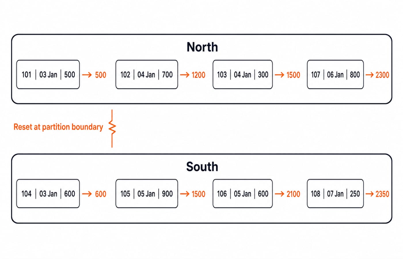
For a row-by-row running total, specify both the sequence and frame:
SUM(amount) OVER (
  PARTITION BY region
  ORDER BY order_date, order_id
  ROWS BETWEEN UNBOUNDED PRECEDING AND CURRENT ROW
) AS running_region_total
North orders 101, 102, 103, 107 produce 500, 1200, 1500, 2300. South orders 104, 105, 106, 108 produce 600, 1500, 2100, 2350.
Use ROW_NUMBER, RANK and DENSE_RANK correctly when values tie
Calculate all three by region, but preserve ties for the two rank functions:
SELECT order_id, region, amount,
  ROW_NUMBER() OVER (
    PARTITION BY region ORDER BY amount DESC, order_id
  ) AS row_number,
  RANK() OVER (
    PARTITION BY region ORDER BY amount DESC
  ) AS rank,
  DENSE_RANK() OVER (
    PARTITION BY region ORDER BY amount DESC
  ) AS dense_rank
FROM sales;
The South result shows the difference clearly:
Order | Amount | ROW_NUMBER | RANK | DENSE_RANK |
|---|---|---|---|---|
105 | 900 | 1 | 1 | 1 |
104 | 600 | 2 | 2 | 2 |
106 | 600 | 3 | 2 | 2 |
108 | 250 | 4 | 4 | 3 |
RANK skips position 3 after the tie. DENSE_RANK does not. Adding order_id inside either rank window would deliberately break the tie.
Use ROW_NUMBER when you need exactly N rows, RANK when tied positions and gaps matter, and DENSE_RANK for the top N distinct values. None is universally better.
Compare rows with LAG and calculate a short moving average
LAG reads an earlier row in the same representative's sequence:
SELECT order_id, rep, amount,
  LAG(amount) OVER (
    PARTITION BY rep ORDER BY order_date, order_id
  ) AS previous_amount,
  amount - LAG(amount) OVER (
    PARTITION BY rep ORDER BY order_date, order_id
  ) AS change_from_previous
FROM sales;
Asha's amounts 500, 300, 800 give changes NULL, -200, +500. Meera's 600, 600 give NULL, 0; Kabir's 900, 250 give NULL, -650; Ravi's single 700 gives NULL. The first row in each partition has no predecessor, so LAG returns NULL unless you supply a default. LEAD applies the same idea looking forward.
A two-row moving average uses the current row and at most one predecessor:
AVG(amount * 1.0) OVER (
  PARTITION BY rep
  ORDER BY order_date, order_id
  ROWS BETWEEN 1 PRECEDING AND CURRENT ROW
) AS moving_average
Asha gets 500.00, 400.00, 550.00; Kabir gets 900.00, 575.00. The first result averages the one available row.
Understand ROWS versus RANGE before trusting a running total
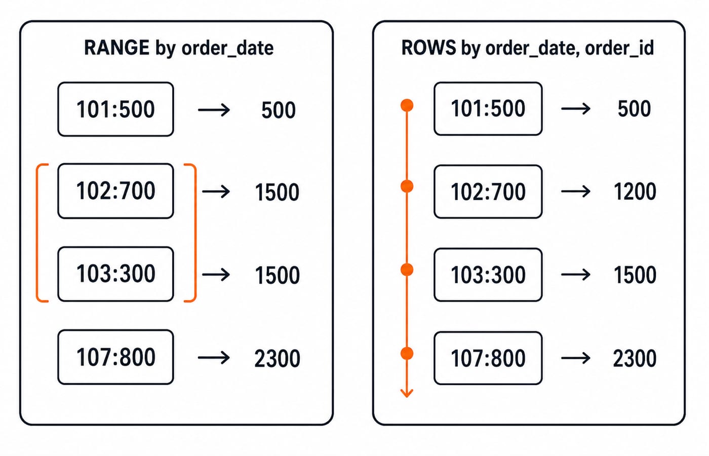
RANGE BETWEEN UNBOUNDED PRECEDING AND CURRENT ROW ordered by order_date treats equal dates as peers. ROWS BETWEEN UNBOUNDED PRECEDING AND CURRENT ROW ordered by order_date, order_id advances one result row at a time.
For North, date-based RANGE gives 500, 1500, 1500, 2300 because orders 102 and 103 share 04 January. Deterministic ROWS gives 500, 1200, 1500, 2300. For South, the 05 January tie makes RANGE produce 600, 2100, 2100, 2350, while ROWS produces 600, 1500, 2100, 2350.
Specify the frame and include a unique tie-breaker when you need a row-by-row total. Choose a peer-aware RANGE frame only when equal sort values should share one cumulative result.
Fix the window-function mistakes that produce wrong or invalid SQL
You cannot normally write WHERE ROW_NUMBER() OVER (...) = 1 in the same query block. WHERE runs before the window result exists. Calculate first, then filter:
WITH ranked AS (
  SELECT *,
    ROW_NUMBER() OVER (
      PARTITION BY region ORDER BY amount DESC, order_id
    ) AS rn
  FROM sales
)
SELECT *
FROM ranked
WHERE rn = 1;
The winners are North order 107, Asha, 800, and South order 105, Kabir, 900.
An unstable ROW_NUMBER ordered only by amount DESC can swap South orders 104 and 106, since both are 600. Add order_id as the final sort key.
LAST_VALUE has another trap. An ordered frame ending at the current row can return the current row, not the partition's last row. To get the actual final sale amount, use ROWS BETWEEN UNBOUNDED PRECEDING AND UNBOUNDED FOLLOWING. Ordered by order_date, order_id, it repeats 800 for North and 250 for South.
Finally, GROUP BY loses detail rows, while an aggregate window without ORDER BY intentionally repeats a partition total. Decide whether you need one row per group or one annotation per original row.
Practise the forms used in SQL interviews and objective tests
For the top two rows per region, calculate ROW_NUMBER() OVER (PARTITION BY region ORDER BY amount DESC, order_id) in a CTE and filter rn <= 2. The result is North 107, 102 and South 105, 104. With DENSE_RANK <= 2, South order 106 also appears because both 600 amounts have the second distinct rank.
For percentage of regional total, calculate:
100.0 * amount / SUM(amount) OVER (PARTITION BY region)North order 107 is 34.78% because 800 / 2300 x 100 = 34.7826.... South order 105 is 38.30% because 900 / 2350 x 100 = 38.2978.... Keep full precision during calculation and round only for display.
One useful diagnosis question is why both 04 January North rows show 1500 under the date-based RANGE frame. They are peers with the same ordering value. The deterministic repair is the explicit ROWS frame ordered by order_date, order_id.
For more query patterns, work through SQL Queries for Placement Interviews, Step by Step. For ranking-focused interview problems, use SQL Window Functions Explained: ROW_NUMBER, RANK, and DENSE_RANK with Interview Problems. Ranking is only one layer; the same sales table also tests partition totals, LAG, moving averages and explicit frames.
Window functions in SQL: the short version and next step
An aggregate plus OVER annotates rows. ROW_NUMBER, RANK and DENSE_RANK order them. LAG and LEAD compare neighbours. An explicit frame defines how much of the partition each row can see.
Use a three-part correctness check: partition the right rows, order ties deterministically, and write the frame explicitly when sequence matters. As practice, change order 106 from 600 to 650. Predict every affected total and rank before running the queries.
Continue with CS Fundamentals for Placements by Sanchit Sir for structured DBMS and placement preparation. If you want a broader multi-subject route, use Zero to Hero: Complete CS Course.
Keep learning

SQL Query Challenges: Window Functions, CTEs and Ranking with Worked Result Sets
Use one 11-row sales table to practise result grain, regional windows, ranking ties, top-N CTEs, running totals and a self-join alternative.
Updated 21 Sep 20266 min readInterview Corner

SQL Window Functions Explained: ROW_NUMBER, RANK, and DENSE_RANK with Interview Problems
See why window functions preserve rows, then calculate three ranking columns on the same tied-score table.
Updated 30 Oct 20265 min read52 viewsDBMS

String Functions in SQL: Clean, Extract and Combine Text with Examples
Build reliable SQL text expressions from small, checkable examples, then combine them into a complete contact-cleaning query with explicit NULL handling.
Updated 9 Nov 20265 min readDBMS

SQL Date Functions: Extract, Add and Filter Dates with Worked Examples
Learn to extract date parts, calculate intervals, write safe timestamp ranges, group monthly data, and translate common operations across four SQL dialects.
Updated 3 Nov 20265 min read51 viewsDBMS