SQL Query Challenges: Window Functions, CTEs and Ranking with Worked Result Sets

A report asks for each sale row, its regional total, regional rank and previous sale. Familiar clauses suddenly stop fitting together. Name the output grain, aggregate only when it must shrink, then add window calculations in a new layer. The 11-row Sale dataset lets you test each intermediate result before running a query.

1. Start every advanced SQL challenge by naming the row grain

Use this practice table: Sale(sale_id PK, rep, region, sale_date, amount). The table contains 11 rows.

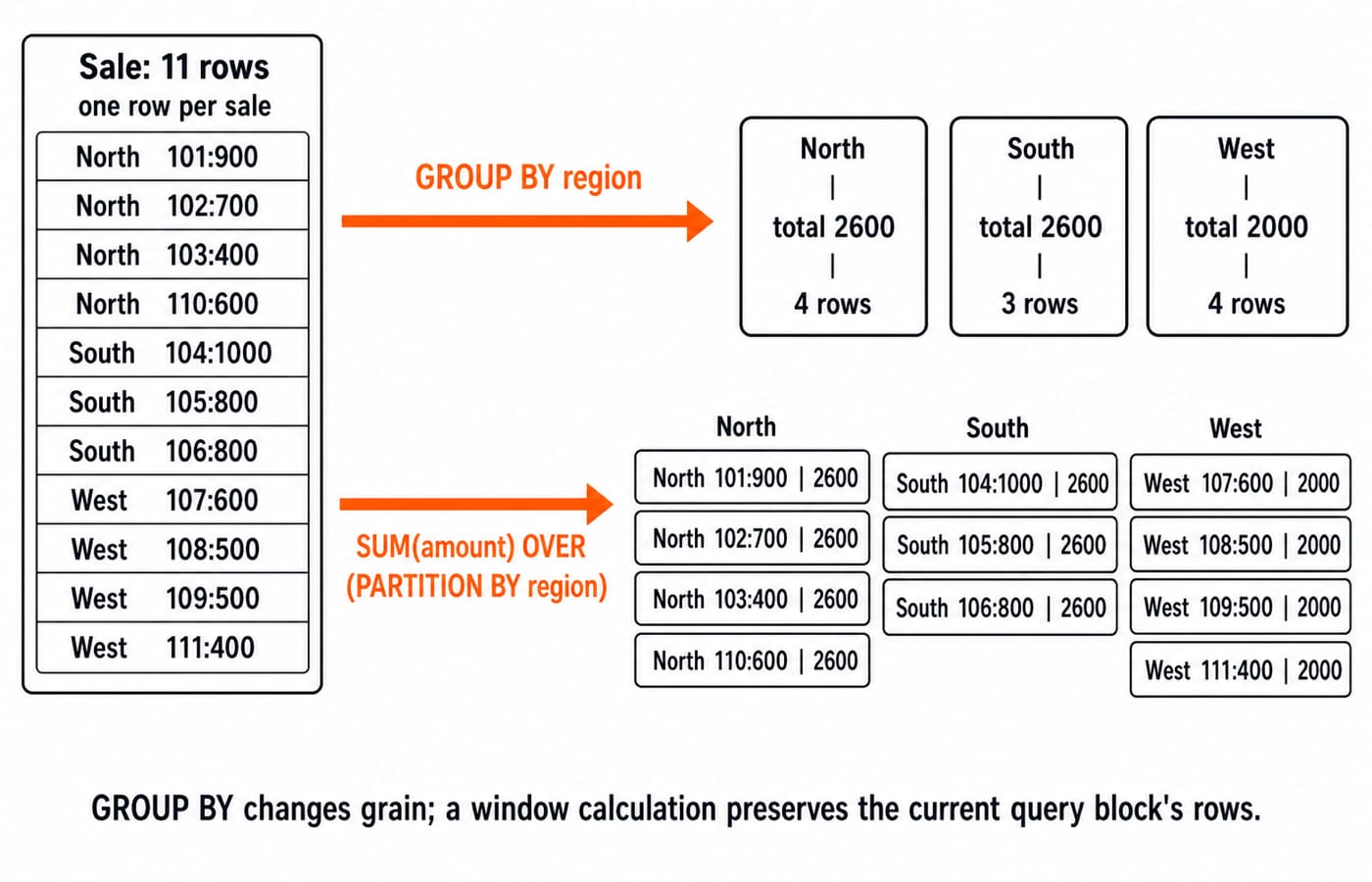
Name the grain before writing SQL. The base table has one row per sale. A regional summary has one row per region. A representative summary has one row per (region, rep); ranking keeps that grain. GROUP BY changes a query block's grain; a window function annotates its existing rows.

For practice with filters, joins and aggregates, start with SQL Queries for Placement Interviews, Step by Step. The Interview & Resume Preparation Course also helps you explain query decisions aloud.

2. GROUP BY versus window aggregates: decide whether rows should collapse

This grouped query returns three rows in no promised order:

SELECT region, SUM(amount) AS region_total, COUNT(*) AS sale_rows
FROM Sale
GROUP BY region;

The 11 sales collapse to region grain, so sale_id and rep cannot be ungrouped output columns. This window query instead returns all 11 rows:

SELECT sale_id, rep, region, amount,
       SUM(amount) OVER (PARTITION BY region) AS region_total
FROM Sale;

Each North and South row carries 2600; each West row carries 2000. Use grouping for three regional rows, or a window aggregate for 11 detail rows with regional totals.

The grand total is 7200. Therefore sale 101 contributes 100.0 * 900 / 7200 = 12.50%, while sale 104 contributes 100.0 * 1000 / 7200 = 13.888...%, about 13.89%. Use decimal-safe division and guard against zero.

3. ROW_NUMBER, RANK and DENSE_RANK: make tie behaviour visible

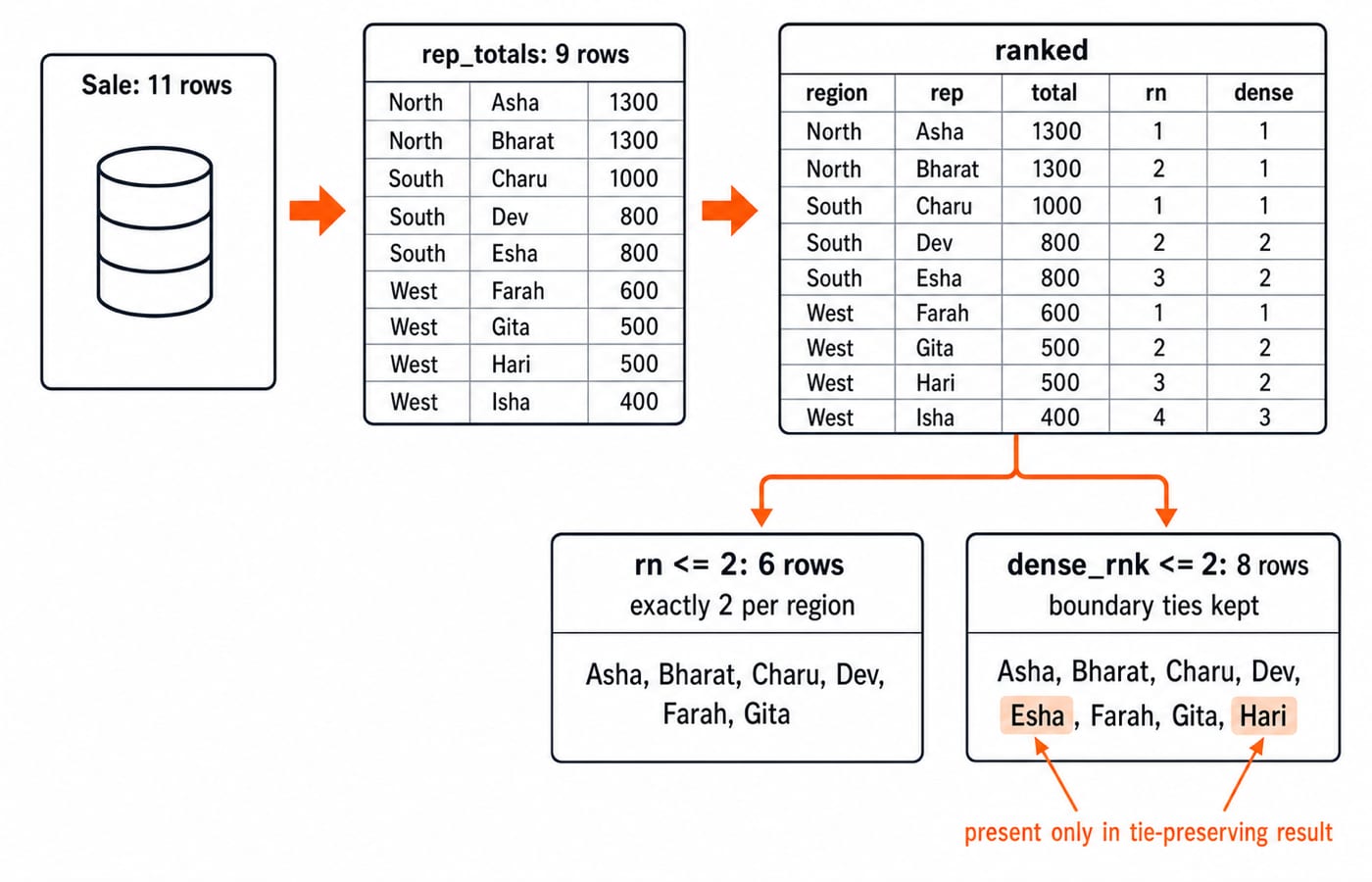
First aggregate with GROUP BY region, rep, then rank the nine totals in a new layer:

Use ROW_NUMBER() OVER (PARTITION BY region ORDER BY total DESC, rep ASC) for unique, deterministic positions. Use RANK() ordered only by total DESC to preserve peers and leave a gap such as 2, 2, 4. DENSE_RANK() preserves peers but continues 2, 2, 3. Do not add rep to the latter two orderings, because that would break the intended amount tie.

4. Build a top-N-per-region report with two CTE layers

The query shape mirrors the reasoning:

WITH rep_totals AS (
  SELECT region, rep, SUM(amount) AS total
  FROM Sale GROUP BY region, rep
), ranked AS (
  SELECT region, rep, total,
    ROW_NUMBER() OVER (PARTITION BY region ORDER BY total DESC, rep ASC) AS rn,
    DENSE_RANK() OVER (PARTITION BY region ORDER BY total DESC) AS dense_rnk
  FROM rep_totals
)
SELECT ... FROM ranked WHERE ...;

The first CTE creates representative rows, the second ranks them, and the outer query filters the rank. WHERE rn <= 2 returns North Asha and Bharat, South Charu and Dev, and West Farah and Gita: six rows, exactly two per region. Esha and Hari lose the alphabetical tiebreaker.

WHERE dense_rnk <= 2 keeps boundary ties: North has Asha and Bharat; South adds Charu, Dev and Esha; West adds Farah, Gita and Hari. That is eight rows. Phrase the requirement first: “exactly two representatives” needs deterministic ROW_NUMBER; “all representatives in the top two distinct totals” needs DENSE_RANK.

5. Running totals, moving frames and LAG on ordered rows

Use explicit ordering and frames:

SELECT sale_id, region, sale_date, amount,
  SUM(amount) OVER (PARTITION BY region ORDER BY sale_date, sale_id
    ROWS BETWEEN UNBOUNDED PRECEDING AND CURRENT ROW) AS running_total,
  SUM(amount) OVER (PARTITION BY region ORDER BY sale_date, sale_id
    ROWS BETWEEN 2 PRECEDING AND CURRENT ROW) AS rolling_3,
  LAG(amount) OVER
    (PARTITION BY region ORDER BY sale_date, sale_id) AS previous_amount
FROM Sale;

sale_id resolves equal-date order.

North traces completely as follows:

For sale 110, rolling three is 700 + 400 + 600 = 1700. Partitioning restarts per region, ordering defines the sequence, and the frame includes the current row plus two preceding rows, not two days. Explicit ROWS avoids ambiguity. Frame defaults and peer handling vary by database, so check its documentation.

6. Compare the window solution with a GROUP BY and self-join

Build the alternative from rep_totals:

SELECT a.region, a.rep, a.total,
       1 + COUNT(DISTINCT b.total) AS dense_position
FROM rep_totals AS a
LEFT JOIN rep_totals AS b
  ON b.region = a.region AND b.total > a.total
GROUP BY a.region, a.rep, a.total;

Asha and Bharat see no greater North total, so both get 1. Dev and Esha see {1000}, so get 2. Gita and Hari see {600}, so get 2. Isha sees {600, 500}, so gets 3.

This reproduces the worked dense ranks by counting distinct greater, non-null totals. Without DISTINCT, repeated higher totals can distort the position. Nulls, collation and extra tie keys need explicit rules. The self-join exposes every comparison but is verbose; DENSE_RANK states the intent. A CTE organises the query but does not promise materialisation or speed, so inspect the engine's plan.

7. Diagnose advanced SQL traps before writing syntax

Predict row counts 3 -> 11 -> 9 -> 6 or 8 for regional totals, detailed window totals, representative ranks, and the two top-N definitions. Then derive North's rolling values. SQL Interview Questions: Joins, GROUP BY and Subqueries with Worked Result Sets owns join expansion, grouped rows and NULL-driven subquery traps. This challenge keeps the result-set method but applies it to window frames, ranking ties and top-N CTEs. Features like QUALIFY, null ordering, date arithmetic and CTE optimisation differ by database, so use its current documentation.

8. Verify every SQL result before running the query

1. Confirm regional totals 2600, 2600 and 2000 at the three-row summary grain.

2. Explain why GROUP BY returns three rows while window SUM preserves all 11 sale rows.

3. Rebuild nine representative totals, then verify the RANK and DENSE_RANK gaps at the West tie.

4. Return six rows with exact-N ROW_NUMBER and eight rows with tie-preserving DENSE_RANK.

5. Derive North running totals 900, 1600, 2000, 2600 and rolling-three totals 900, 1600, 2000, 1700, then check the self-join dense positions.

Before leaving the dataset, check five things: the output grain, the aggregation layer, the ranking or comparison layer, the tie rule and the predicted row count. For broader revision, CS Fundamentals for Placements by Sanchit Sir covers SQL and DBMS. The Resume & Interview Preparation category offers broader interview practice.