

Raster Scan vs Random Scan: Concepts, Worked Examples and Exam Traps
Learn what each display model stores and refreshes, then work through line sampling, frame-buffer memory, and primitive-based refresh calculations.
KnowledgeGate Team
Exam prep & CS education
Updated 16 Nov 20265 min read

Both systems can draw a line. The useful distinction is what each stores and which path it refreshes. Coordinate and workload calculations distinguish the two classical textbook models.
Raster Scan vs Random Scan in One View
Raster scan treats the screen as a rectangular pixel grid refreshed line by line. Random scan, also called vector or calligraphic scan, uses a display list to direct the beam along selected primitives.
Raster work follows pixel count and colour depth. Classical random-scan work follows the number and complexity of listed primitives. Keep this distinction precise alongside other CS Fundamentals.
Feature | Raster scan | Classical random scan |
|---|---|---|
Stored representation | Pixel values in a frame buffer | Commands in a display list |
Refresh path | Every row in sequence | Listed primitives only |
Best-suited image type | Filled and realistic images | Sparse lines and wireframes |
Line appearance | Pixel samples can alias | Smooth classical traces |
Filled or shaded areas | Natural per-pixel representation | Awkward to trace densely |
Main memory driver | Resolution × colour depth | Primitive count and description |
Main complexity limit | Pixel and bandwidth costs | Full-list redraw time |
How a Raster-Scan Display Builds and Refreshes an Image
An application produces primitives, rasterisation selects pixel samples, the frame buffer stores their values, and the display scans rows top to bottom. Lines and curves must be sampled onto the grid. The resulting stair-step edges are aliasing; resolution and antialiasing can reduce them.
The reusable memory formula is:
frame-buffer bits = horizontal pixels × vertical pixels × bits per pixel
Divide by 8 for bytes. Resolution sets pixel count, colour depth sets bits per pixel, and refresh rate sets how often a frame is read.
This classical exam model does not imply that every modern flat panel contains a moving electron beam.
How a Random-Scan Display Uses a Display List
The picture might store MOVE (2,2) and DRAW (10,6). The system moves, traces the line, processes the next command, then repeats the list to maintain the picture.
Direct tracing gives smooth straight wireframes. Filled regions, shading, photographs and dense scenes need many traces. A larger primitive list takes longer to redraw, reducing the achievable refresh rate.
Random scan is historically important and exam-relevant, not the standard architecture of current general-purpose displays.
Worked Example 1: Draw the Same Line on Both Systems
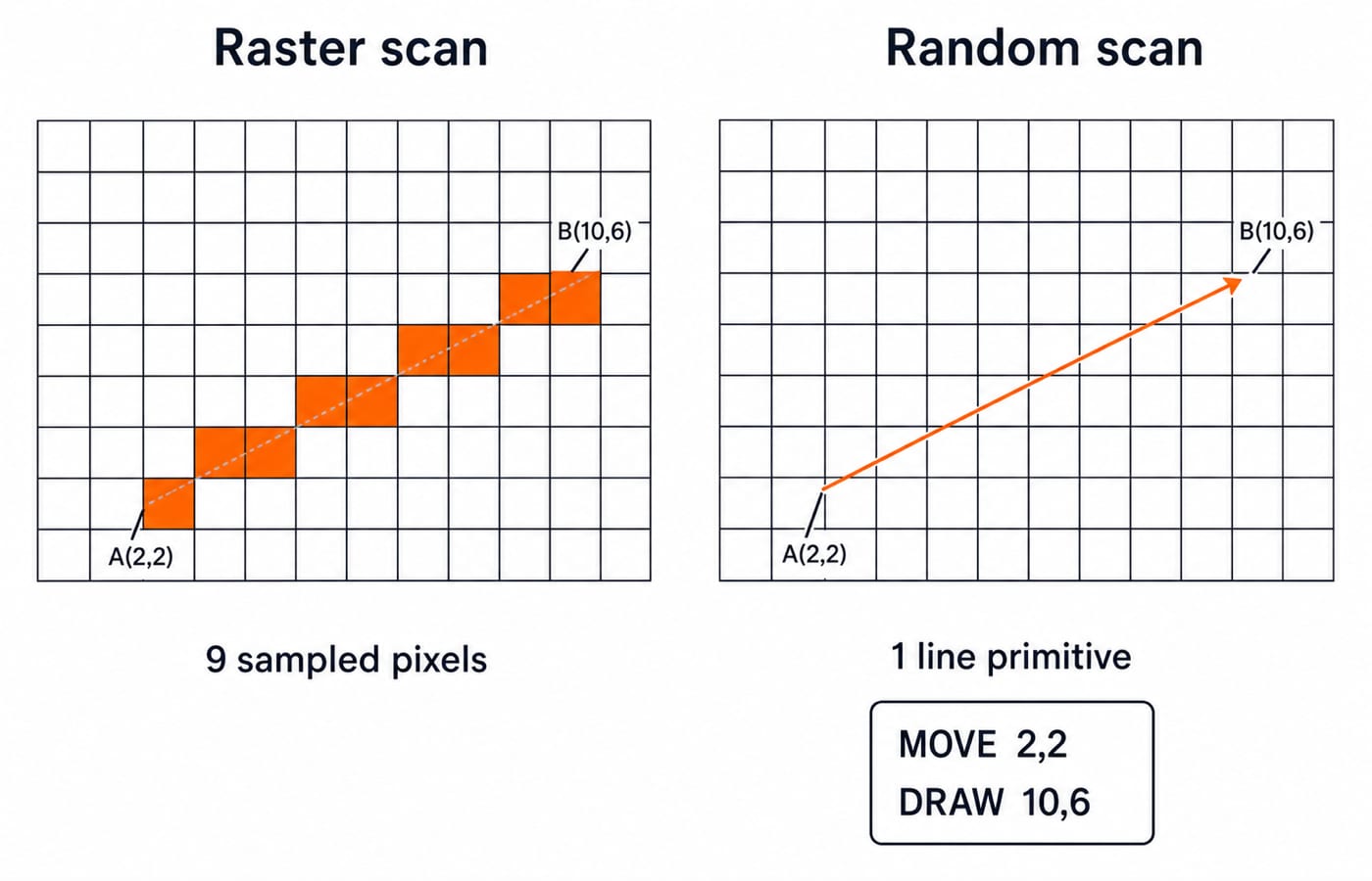
Take a 12 × 8 coordinate field and the segment from A(2,2) to B(10,6). Its slope is:
m = (6 - 2) / (10 - 2) = 4 / 8 = 0.5
Here dx = 8, dy = 4, and the initial Bresenham decision is p0 = 2dy - dx = 8 - 8 = 0. With p >= 0 choosing north-east, the cells are:
(2,2), (3,3), (4,3), (5,4), (6,4), (7,5), (8,5), (9,6), (10,6)
Raster stores nine samples. Random scan stores and traces one line primitive from A to B. The intended geometry is the same, but its representation differs.
Another documented tie rule may choose the other close pixel. Our rule removes ambiguity.
Worked Example 2: Frame-Buffer Memory and Refresh Work
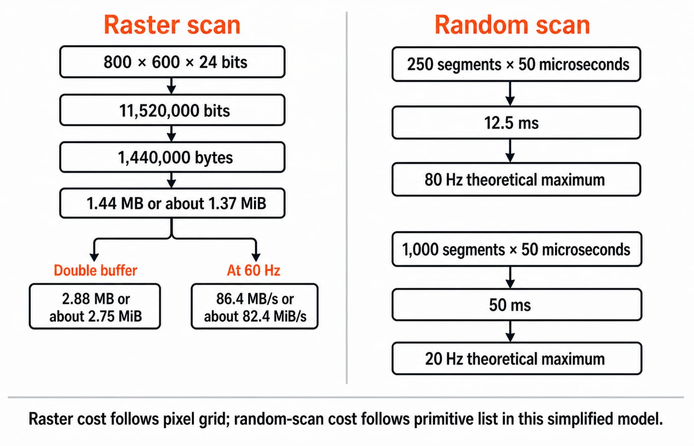
For 800 × 600 pixels at 24 bits/pixel:
800 × 600 × 24 = 11,520,000 bits.11,520,000 ÷ 8 = 1,440,000 bytes.That is
1.44 MBin decimal units, approximately1.37 MiB.A double buffer needs
2,880,000 bytes = 2.88 MB, approximately2.75 MiB.
At 60 refreshes per second, a simplified raw frame read is:
1,440,000 × 60 = 86,400,000 bytes/second
That is 86.4 MB/s, approximately 82.4 MiB/s. This teaching calculation ignores compression, blanking, protocol overhead and implementation details. The earlier Computer Graphics Fundamentals: Applications, Core Components and a Worked Pixel Pipeline article owns the component chain, triangle pipeline, and combined colour-and-depth-buffer calculation. This comparison isolates scan-system representation, line sampling, and primitive-list refresh cost.
For 250 random-scan line segments at 50 microseconds each:
250 × 50 microseconds = 12,500 microseconds = 12.5 ms
The theoretical ceiling is 1 / 0.0125 = 80 refreshes/second. At 1,000 segments, 1,000 × 50 = 50,000 microseconds = 50 ms, giving 1 / 0.05 = 20 refreshes/second. Real overhead lowers both rates.
Which System Fits Which Image, and Why
A 120-edge CAD wireframe suits classical random scan as a small line list. A 1920 × 1080 photograph needs raster-style pixel colour. A dashboard with text, icons, filled charts and images is naturally rasterised, even when shapes begin as vectors.
Vector artwork and random scan are not synonyms. Vector files can be rasterised, and raster screens can show excellent antialiased lines.
Use four questions to classify a case:
Is the content mostly sparse lines, or does it contain filled and realistic imagery?
Is independent colour needed at each pixel?
Does storage grow mainly with the pixel grid or with the primitive list?
Does redraw time grow as more primitives are added?
Exam Patterns and Traps
Exams often ask you to identify a refresh description, match properties, calculate buffer memory, or find a primitive limit. At 40 microseconds per segment and 50 Hz minimum, the budget is 1 / 50 = 20 ms = 20,000 microseconds. The simplified maximum is 20,000 / 40 = 500 segments before overhead.
Watch for these traps:
Random does not mean unpredictable. It means following selected primitives instead of a fixed row order.
Raster scan can draw lines. It rasterises them into pixel samples.
Random scan does not mean zero memory. It needs a display list and supporting state.
Bits are not bytes. Divide by 8 before reporting byte capacity.
MB and MiB differ. Decimal MB uses powers of 1,000; binary MiB uses powers of 1,024.
Refresh time depends on scene complexity. More primitives take longer to redraw.
These are common styles, not an official blueprint. Confirm the current syllabus and pattern on the exam body's official site. For another timing numerical, read Pipelining in Computer Architecture.
Short Version and Next Step
Raster scan stores pixel values and refreshes the whole grid.
Random scan stores geometric commands and traces selected primitives.
Raster scan handles filled, shaded and realistic images well.
Classical random scan suits sparse line drawings, but slows as its display list grows.
In ten minutes, recompute the 800 × 600 × 24-bit example, solve the 500-segment variation, and redraw A to B from memory.
For structured study, ZERO TO HERO offers a broad, semester-oriented CS path. Computer Science Fundamentals for Placements focuses on placements.
Keep learning

Raster vs Random Scan MCQs and Descriptive Problems: Solved Questions with Explanations
Attempt seven option-based questions and four descriptive problems on raster and random scan systems, then check each answer with a compact explanation.
Updated 23 Sep 20267 min readTeaching Recruitment (Computer Science)

Random Variables and Distributions for GATE CS: Expectation and Variance Numericals Solved
Compute expectation and variance from a PMF, recognise four standard distributions, and use linearity and variance scaling without silent formula errors.
Updated 8 Sep 20265 min read83 viewsGATE Strategy & Roadmap
Display Technologies MCQs: 12 Solved CRT, LCD and Raster Questions
Practise 12 display-technology questions on aspect ratio, CRT parts, phosphor behaviour, raster scanning and LCD layers, with answers and clear explanations.
Updated 29 Oct 20266 min readUGC NET Computer Science

Display Technologies Explained: CRT, LCD, LED and OLED with Worked Raster Numericals
Follow a pixel from the frame buffer to the screen, compare scanning with flat-panel addressing, and check two complete raster calculations.
Updated 6 Sep 20266 min readUGC NET Computer Science