

Gradient Descent for Linear Regression: Derive and Run One Update by Hand
See prediction, residual, gradient and parameter update as one continuous calculation. Then verify the lower loss and test what an oversized learning rate does.
KnowledgeGate Team
Exam prep & CS education
Updated 17 Nov 20265 min read
You can call an optimiser in one line, yet its returned parameters may feel arbitrary because prediction, error, gradient and update are hidden inside that call. For the points (1,2) and (2,3), starting from w=0.5, b=0.5 with alpha=0.1, the complete calculation shows prediction, error, gradient and update explicitly. One verified update gives (w,b)=(0.7,0.625) and lowers the cost from 0.8125 to 0.3515625.
Gradient descent starts with a model, an error and one exact cost function
For example i, y_hat_i = w x_i + b, where w is the slope, b the intercept, y_hat_i the prediction and y_i the target. Define e_i = y_hat_i - y_i, always prediction minus target. Changing this sign without changing the derivative reverses the update.
For m examples, use the full-batch objective
J(w,b) = (1/(2m)) Σ_i e_i^2 = (1/(2m)) Σ_i (w x_i + b - y_i)^2.
The term e_i^2 belongs to one example; J covers the dataset. Squaring stops opposite residuals from cancelling. The factor 1/2 only cancels the 2 from differentiation and does not change the minimising parameters.
Let theta=(w,b) and grad J=(partial J/partial w, partial J/partial b). Since the gradient points towards steepest local increase, descent moves opposite it. Coding & Skills covers broader programming, AI and machine-learning study.
Derive the linear-regression gradient with the chain rule
For the slope component, retain the inner derivative:
partial J/partial w = (1/(2m)) Σ_i 2e_i (partial e_i/partial w).
Since e_i = w x_i + b - y_i, partial e_i/partial w = x_i. Cancelling the 2 gives
partial J/partial w = (1/m) Σ_i e_i x_i.
For the same residual, an example with a larger x_i contributes proportionally more to the slope gradient. For the intercept, partial e_i/partial b = 1, so
partial J/partial b = (1/m) Σ_i e_i.
Therefore, grad J = ((1/m) Σ_i e_i x_i, (1/m) Σ_i e_i). Update the two parameters simultaneously:
w_new = w_old - alpha(partial J/partial w)
b_new = b_old - alpha(partial J/partial b)
Evaluate both gradients at the same old (w,b). Do not update w before calculating the gradient for b. Optimisation is one mechanism in the wider Approaches to AI map, but not every AI approach trains this model.
Run the forward pass at w=0.5 and b=0.5
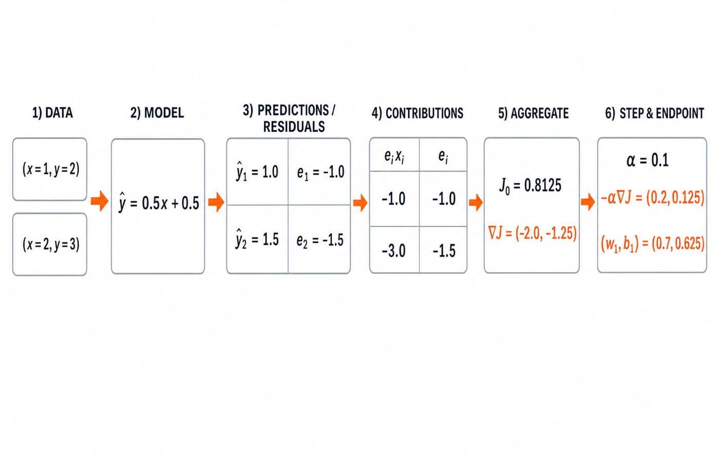
Using both points together, the predictions are 0.5(1)+0.5=1.0 and 0.5(2)+0.5=1.5. This forward pass does not change parameters. It records the outputs needed for the cost and gradient, all from the same old values.
i | x_i | y_i | y_hat_i | e_i | e_i^2 | e_i x_i |
|---|---|---|---|---|---|---|
1 | 1 | 2 | 1.0 | -1.0 | 1.0 | -1.0 |
2 | 2 | 3 | 1.5 | -1.5 | 2.25 | -3.0 |
With m=2, the starting cost is
J_0 = (1/(2 × 2))[(-1)^2+(-1.5)^2]
= (1/4)(1+2.25) = 3.25/4 = 0.8125.
The denominator is 2m=4, so 1.625 is not our cost. Both predictions are low, so their residuals are negative. Positive inputs make both e_i x_i terms negative too. Subtracting the resulting negative derivatives will increase both parameters.
Calculate the gradient and complete one simultaneous update
Aggregate the contribution columns from the forward pass:
partial J/partial w = [(-1.0)+(-3.0)]/2 = -4/2 = -2.0
partial J/partial b = [(-1.0)+(-1.5)]/2 = -2.5/2 = -1.25
Thus, grad J(0.5,0.5)=(-2.0,-1.25). Apply alpha=0.1 to both old parameter values:
w_1 = 0.5 - 0.1(-2.0) = 0.7
b_1 = 0.5 - 0.1(-1.25) = 0.625
In vector form, Delta theta = -alpha grad J = (0.2,0.125) and (0.5,0.5)+(0.2,0.125)=(0.7,0.625). Both components came from the gradient at (0.5,0.5), so the update is simultaneous.
The direction makes sense: the starting line underpredicts both targets, so raising its slope and intercept is sensible. Algebra reaches the same conclusion when a model has too many parameters to picture.
Verify the update by recomputing the loss
Now run the same two examples through (w_1,b_1)=(0.7,0.625).
This second forward pass is the simplest practical audit. It tests the updated model against the same cost definition instead of assuming that an update helped.
i | Calculation | y_hat_i | e_i | e_i^2 |
|---|---|---|---|---|
1 |
| 1.325 | -0.675 | 0.455625 |
2 |
| 2.025 | -0.975 | 0.950625 |
Recompute the objective independently:
J_1 = (1/4)(0.455625+0.950625)
= (1/4)(1.40625) = 0.3515625.
The cost falls from 0.8125 to 0.3515625. The absolute drop is 0.4609375; the relative reduction is (0.4609375/0.8125) × 100, about 56.73%. This describes the toy step, not every dataset or iteration.
As an audit, the new gradient is ([(-0.675)(1)+(-0.975)(2)]/2, [-0.675-0.975]/2) = (-1.3125,-0.825). Its norm, about 1.5503, is below the starting 2.3585. That fits a flatter local slope here, but does not prove convergence generally.
The learning rate decides whether the same gradient helps or overshoots
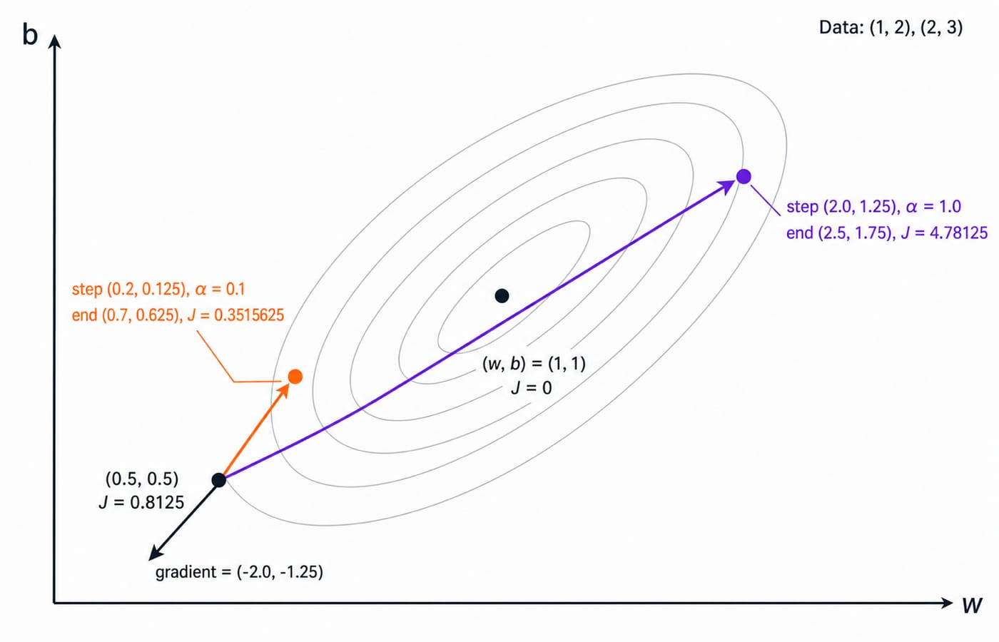
Reuse the starting gradient (-2.0,-1.25), but deliberately set alpha=1.0. Then w=0.5-1(-2)=2.5 and b=0.5-1(-1.25)=1.75. The predictions become 4.25 and 6.75, so the residuals are 2.25 and 3.75. The resulting cost is
J = (1/4)(2.25^2+3.75^2) = (1/4)(5.0625+14.0625) = 4.78125.
The one-step increase to 4.78125 signals overshoot, and repeated oversized steps can diverge. A very small positive alpha usually gives slow progress. A suitable value can decrease this smooth convex quadratic. An oversized value can cross its valley and increase loss. This does not promise that every step decreases an arbitrary non-convex objective.
For an exact check, design rows (x_i,1) give Hessian (1/m)X^T X = [[2.5,1.5],[1.5,1]]. Its largest eigenvalue is about 3.4271, so fixed-step descent on this quadratic converges for 0<alpha<2/3.4271, about 0.5836. Thus 0.1 is inside and 1.0 outside.
Gradient descent traps and assessment-style checks
Wrong move | What goes wrong | Correct move |
|---|---|---|
Use | Reversed gradient sign | Keep one residual convention |
Forget division by | Wrong gradient scale | Average both sums over |
Mix plain MSE with the defined | Loss and derivative disagree | Keep the stated cost convention |
Update | The step stops being simultaneous | Calculate both components at old |
Move with | Parameters move uphill | Use |
Try three short checks:
If
grad J=(3,-4),theta=(2,1)andalpha=0.05, thentheta_new=(2,1)-0.05(3,-4)=(1.85,1.20).Starting from the initial parameters, alpha=0.05 gives (w,b)=(0.6,0.5625).
A zero gradient can mark a minimum, maximum, saddle point or flat region in a general objective. This full-rank linear-regression quadratic has the unique minimum
(1,1).
For adjacent learned-model practice, use Artificial Neural Networks MCQs: 10 Solved Questions with Explanations.
Gradient descent short version and the next step
Keep this six-line chain:
Predict with
y_hat=wx+b.Form
e=y_hat-y.Calculate
J=(1/(2m))Σe^2.Derive
grad J=((1/m)Σex,(1/m)Σe).Update both parameters with
theta_new=theta_old-alpha grad J.Recompute the loss before calling the step useful.
Here (0.5,0.5) becomes (0.7,0.625), and J falls to 0.3515625. Cover the table and reproduce both gradient components from the raw points. Then use alpha=0.05 and confirm (0.6,0.5625) before checking the solution. For a broader next learning path, explore Artificial Intelligence (AI) as you move from one hand-computed optimiser step towards wider AI and machine-learning study.
Keep learning

Gradient Boosting Regression: Build Two Residual-Correcting Trees Step by Step
See every stage of gradient boosting regression on five data points, from the initial mean through two residual-fitted stumps and their additive predictions.
Updated 16 Nov 20266 min readML & Data Science

Top-Down Parsing in Compiler Design: Recursive Descent, LL(1), FIRST and FOLLOW with Worked Examples
Learn top-down parsing from grammar preparation to predictive parsing, with one expression grammar carried through every calculation and trace.
Updated 17 Aug 20267 min read148 viewsCompiler Design

Maximum Likelihood Estimation for a Bernoulli Model: Fit p by Hand
See why the Bernoulli MLE is the sample proportion. One eight-observation example builds the likelihood, solves it, and checks the result.
Updated 12 Nov 20265 min readML & Data Science

Recursion in C: Stack Frames, a Hand-Tracing Method and Solved GATE Questions
Trace recursive C programs without guessing. Follow factorial returns, prints on descent and unwind, Fibonacci call counts, and maximum stack depth.
Updated 30 Oct 20267 min readDSA & Algorithms