

LJF and HRRN CPU Scheduling: Worked Gantt Charts, Formula and Exam Traps
Solve one five-process data set under non-preemptive LJF and HRRN, then compare every completion, turnaround, and waiting time.
KnowledgeGate Team
Exam prep & CS education
Updated 4 Nov 20266 min read

LJF looks like a one-line rule, and HRRN like a one-line formula. The difficulty is rebuilding the ready queue only at dispatch times, using current waiting time, and separating arrival, burst, completion, turnaround, and waiting time. In the five-process workload below, LJF postpones a short job while HRRN changes the dispatch order as waiting grows. For context, review the wider CPU scheduling algorithm family.
LJF and HRRN: define the scheduling decisions precisely
Assume one CPU, non-preemptive execution, zero context-switch cost, and known arrival AT and burst BT. At completion, the ready set includes only processes with AT <= current time. The selection runs to completion.
Longest Job First (LJF) chooses the largest original burst among ready processes. Highest Response Ratio Next (HRRN) chooses the largest
RR = (waiting time + burst time) / burst time = 1 + waiting time / burst time.
Recompute HRRN at every dispatch. Break ties by earlier arrival, then smaller process ID.
Policy | Selection key | Preemptive here? | What changes while waiting? | Main risk or benefit |
|---|---|---|---|---|
LJF | Largest | No | Nothing in the key | Short jobs can be postponed |
HRRN | Largest | No |
| Ageing reduces starvation risk |
LRTF or LRJF is different: it makes preemptive decisions using remaining time.
LJF worked example: schedule the longest ready burst
The process set is:
Process | AT | BT |
|---|---|---|
P1 | 0 | 4 |
P2 | 1 | 8 |
P3 | 2 | 2 |
P4 | 3 | 6 |
P5 | 5 | 3 |
Keep the assumptions and tie rule. After scheduling, use CT = completion time, TAT = CT - AT, and WT = TAT - BT.
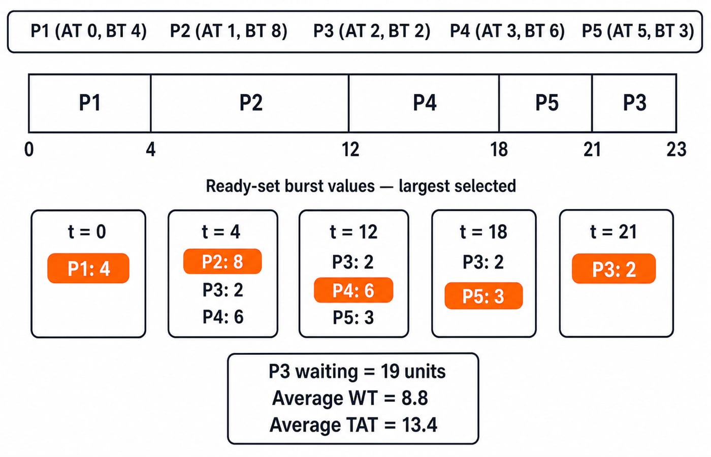
t=0: only P1 is ready. Run it from0to4.t=4: ready P2(8), P3(2), P4(6). Run P2 from4to12.t=12: ready P3(2), P4(6), P5(3). Run P4 from12to18.Run P5 from
18to21, then P3 from21to23.
The LJF Gantt order is 0 | P1 | 4 | P2 | 12 | P4 | 18 | P5 | 21 | P3 | 23.
Process | CT | TAT | WT |
|---|---|---|---|
P1 | 4 |
|
|
P2 | 12 |
|
|
P3 | 23 |
|
|
P4 | 18 |
|
|
P5 | 21 |
|
|
Sum WT = 0 + 3 + 19 + 9 + 13 = 44; average WT is 44/5 = 8.8. Sum TAT = 4 + 11 + 21 + 15 + 16 = 67; average TAT is 67/5 = 13.4.
HRRN worked example: recompute at every dispatch
At t=0, only P1 is ready, so it runs from 0 to 4.
At t=4:
P2:
W = 4 - 1 = 3, soRR = (3 + 8)/8 = 11/8 = 1.375.P3:
W = 4 - 2 = 2, soRR = (2 + 2)/2 = 2.P4:
W = 4 - 3 = 1, soRR = (1 + 6)/6 = 7/6, about1.167.
P3 runs from 4 to 6. At t=6, recompute: P2 has W=5, RR=13/8=1.625; P4 has W=3, RR=9/6=1.5; P5 has W=1, RR=4/3, about 1.333. Select P2 for 6 to 14.
At t=14, P4 has W=11, RR=17/6, about 2.833; P5 has W=9, RR=12/3=4. Run P5 from 14 to 17. At t=17, only P4 remains, with W=14, RR=20/6, about 3.333; run it to 23.
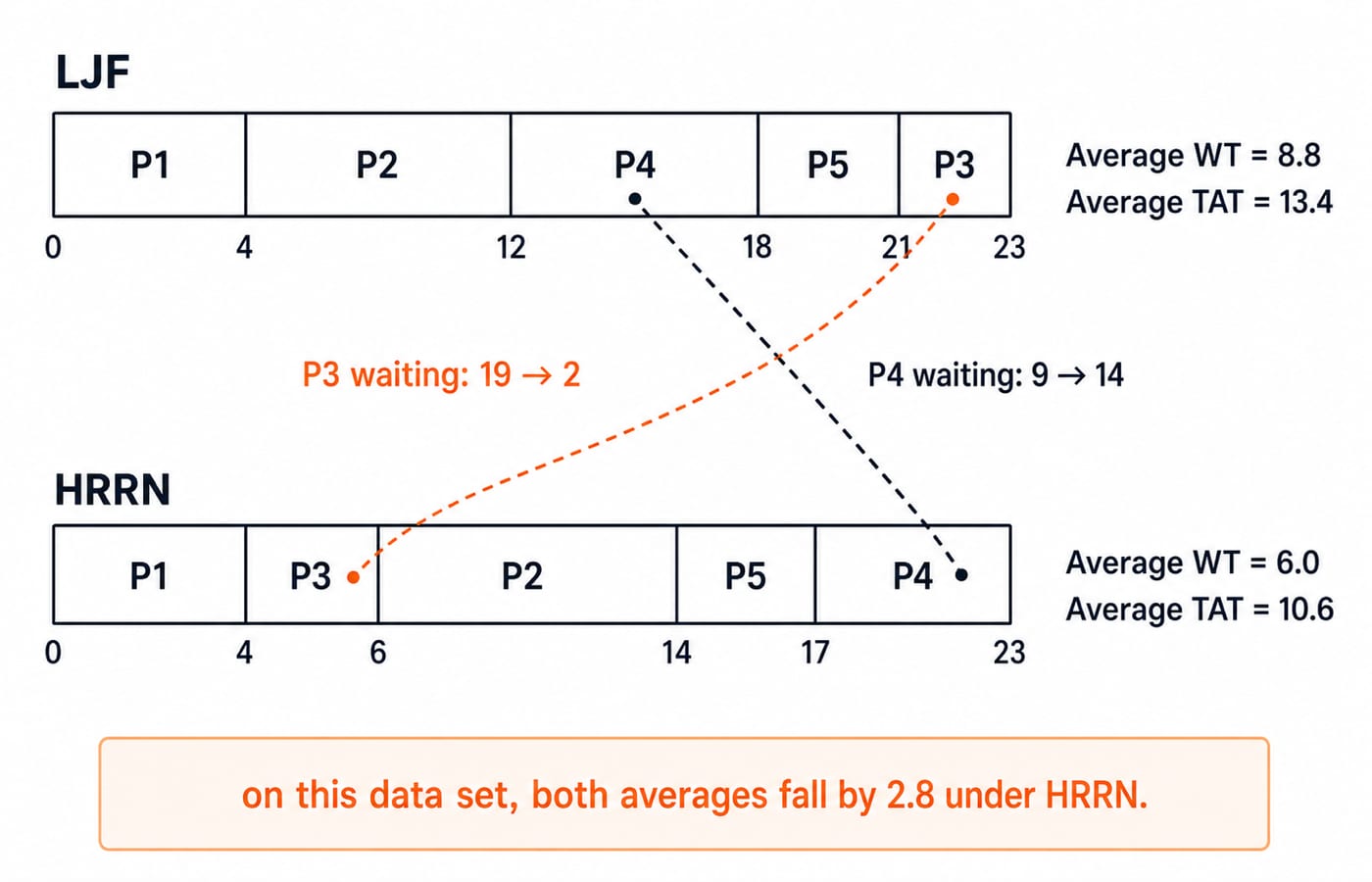
The HRRN order is 0 | P1 | 4 | P3 | 6 | P2 | 14 | P5 | 17 | P4 | 23. Longer bursts do not automatically win because waiting changes each ratio.
LJF versus HRRN: compare the completed schedules
Process | HRRN CT | HRRN TAT | HRRN WT |
|---|---|---|---|
P1 | 4 |
|
|
P2 | 14 |
|
|
P3 | 6 |
|
|
P4 | 23 |
|
|
P5 | 17 |
|
|
For HRRN, sum WT = 0 + 5 + 2 + 14 + 9 = 30; average WT is 30/5 = 6.0. Sum TAT = 4 + 13 + 4 + 20 + 12 = 53; average TAT is 53/5 = 10.6.
Policy | Order | Average WT | Average TAT |
|---|---|---|---|
LJF | P1, P2, P4, P5, P3 | 8.8 | 13.4 |
HRRN | P1, P3, P2, P5, P4 | 6.0 | 10.6 |
Here, HRRN lowers both averages by 2.8: 8.8 - 6.0 = 2.8 and 13.4 - 10.6 = 2.8. P3's WT falls from 19 to 2, while P4's rises from 9 to 14. It does not follow that HRRN always minimises either average.
HRRN ageing and LJF starvation risk
The formula RR = 1 + W/BT explains ageing. A new job starts at ratio 1. As W grows, a short job's ratio rises faster because W is divided by BT.
Under LJF, P3 is ready at t=2 but loses at t=4 to P2(8), at t=12 to P4(6), and at t=18 to P5(3). It starts at t=21 and waits 21 - 2 = 19. Under HRRN, its ratio at t=4 is 2, above P2's 1.375 and P4's roughly 1.167, so it waits only 2.
Every process completes here. With continuing arrivals, LJF can postpone a short job. HRRN's ageing reduces that risk without guaranteeing fairness or optimal averages.
LJF and HRRN traps that change the answer
Wrong move | Correction |
|---|---|
Choose the globally longest process | Choose the longest process already arrived |
Recalculate LJF during a burst | This version is non-preemptive, so wait for completion |
Treat LJF and LRTF as identical | LJF uses original burst at dispatch; LRTF uses remaining time preemptively |
Use turnaround time in HRRN's numerator | Use current waiting time plus burst time |
Compute each HRRN ratio once | Recompute at every dispatch |
Use remaining time as HRRN service time | Use the original burst because an unselected process has not run |
Include P5 at | P5 arrives at |
Take CT from the chart, then use TAT=CT-AT and WT=TAT-BT. WT is not start time when arrival is non-zero. If no job is ready, show an idle interval until the next arrival. Zero context-switch cost is only an assumption here. With simultaneous arrivals, every initial HRRN ratio is 1, so the tie rule decides.
How exam-style questions test LJF and HRRN
Questions may ask for a Gantt chart, metrics, an HRRN dispatch, LJF versus LRTF, starvation, non-preemption, a tie, or an idle interval. For mixed scheduling practice, try Process Scheduling MCQs: 12 Solved.
Use this sequence: note time, exclude future arrivals, form the ready set, compute the key, apply the tie rule, append the burst, and repeat. Then derive metrics from CT. Check LJF with sum WT=44, sum TAT=67, and HRRN with sum WT=30, sum TAT=53.
At t=10, let A have AT=2, BT=4, B have AT=6, BT=2, and C have AT=9, BT=8. LJF selects C. For HRRN, A has W=8, RR=12/4=3; B has W=4, RR=6/2=3; C has W=1, RR=9/8=1.125. A and B tie, so earlier arrival selects A. Without a tie rule, the answer is ambiguous. Use the GATE Test Series for timed practice.
LJF and HRRN: the short version and next step
LJF selects the largest ready burst; HRRN selects the largest 1 + W/BT. Both are non-preemptive here. Filter arrivals before selecting and derive metrics after the chart. The schedules are P1-P2-P4-P5-P3 for LJF and P1-P3-P2-P5-P4 for HRRN.
Hide the tables, redraw both charts, and confirm that P3 waits 19 under LJF and 2 under HRRN. If not, inspect LJF at t=4, 12, 18, or recompute HRRN at t=4, 6, 14.
For a structured core-CS path, use GATE Guidance by Sanchit Sir. Browse GATE CS Exam Preparation for the broader catalogue, or use the GATE Test Series for timed practice.
Go deeper with the full courseOperating System
Keep learning

CPU Scheduling in Operating Systems: Algorithms, Gantt Charts and Worked Examples
Trace one process set through five CPU scheduling policies, calculate every core metric, and extend the method to switching costs and MLFQ.
Updated 17 Aug 20266 min read66 viewsOperating Systems
SJF and SRTF Scheduling: Concepts, Gantt Charts and Worked Examples
Learn how non-preemptive SJF and preemptive SRTF schedule the same four processes, then calculate CT, TAT and WT while avoiding arrival, tie and Gantt-chart traps.
Updated 8 Nov 20265 min readOperating Systems

FCFS Scheduling: Gantt Charts, Waiting Time and Exam Traps
Learn FCFS scheduling through a four-process trace, a complete metric table, convoy-effect reasoning, and checks for idle time, ties and context switches.
Updated 2 Nov 20265 min readOperating Systems

Round Robin Scheduling Explained: Gantt Charts, Waiting Time and GATE Traps
Learn a fixed Round Robin queue convention, trace staggered arrivals, calculate CT, TAT, WT and RT, and see how quantum size and context-switch cost change results.
Updated 9 Oct 20265 min read128 viewsOperating Systems