CPU Scheduling in Operating Systems: Algorithms, Gantt Charts and Worked Examples
Trace one process set through five CPU scheduling policies, calculate every core metric, and extend the method to switching costs and MLFQ.
KnowledgeGate Team
Exam prep & CS education
Updated 17 Aug 20266 min read
CPU scheduling is easy to memorise as five names and easy to get wrong when an arrival, preemption or ready-queue tie changes the Gantt chart. The chart produces every completion, turnaround, waiting and response answer, so method matters more than acronym. One four-process set, with bursts 8, 4, 9 and 5 arriving at times 0, 1, 2 and 3, behaves very differently under FCFS, SJF, SRTF, preemptive Priority and Round Robin: its average waiting time swings from 6.5 to 13.5 on the policy alone. Starvation, ageing and multilevel feedback queues follow from the same arithmetic.
CPU scheduling inside process execution
A process alternates between CPU bursts and I/O waits. After I/O completes, it returns to the ready queue, which contains in-memory processes ready to run. CPU-bound work tends to have longer bursts, while interactive work needs quick response.
The long-term scheduler controls admission and multiprogramming. The medium-term scheduler may suspend and resume work. The short-term scheduler selects the next ready process, while the dispatcher switches context, enters user mode and transfers control. Dispatch latency is overhead.
Decision points are running to waiting, running to ready, waiting to ready, and termination. A non-preemptive policy retains the CPU until blocking or termination. A preemptive policy may also reconsider after a timer expiry or higher-ranked arrival.
CPU scheduling criteria and the arithmetic behind every answer
Let arrival time be AT, total burst be BT, first start be ST, and completion be CT:
TAT = CT - AT
WT = TAT - BT
RT = ST - AT
These formulas assume BT is total CPU service. With separate I/O bursts, follow the question's waiting definition.
CPU utilisation is useful work divided by elapsed time; throughput is completions per time unit. Turnaround spans arrival to completion, waiting covers the ready queue, and response ends at first allocation. For AT=2, ST=5, BT=6, CT=14: RT=3, TAT=12, and WT=6. Response differs from waiting because a preempted process may wait again.
SJF usually predicts its next burst. Using tau_(n+1) = alpha*t_n + (1-alpha)*tau_n, let alpha=0.5, old prediction 6 ms, and actual burst 10 ms. The next prediction is 8 ms; after an actual 4 ms, it becomes 0.5(4) + 0.5(8) = 6 ms. Prediction is not a guarantee.
FCFS, SJF and SRTF on one process set
Use one CPU, no I/O, zero switch cost, smaller priority number as higher priority, and break equal ranks by earlier arrival, then process ID.
Process | AT | BT | Priority |
|---|---|---|---|
P1 | 0 | 8 | 2 |
P2 | 1 | 4 | 1 |
P3 | 2 | 9 | 3 |
P4 | 3 | 5 | 2 |
Policy | Gantt trace | CT | TAT | WT | RT |
|---|---|---|---|---|---|
FCFS |
|
|
|
|
|
SJF |
|
|
|
|
|
SRTF |
|
|
|
|
|
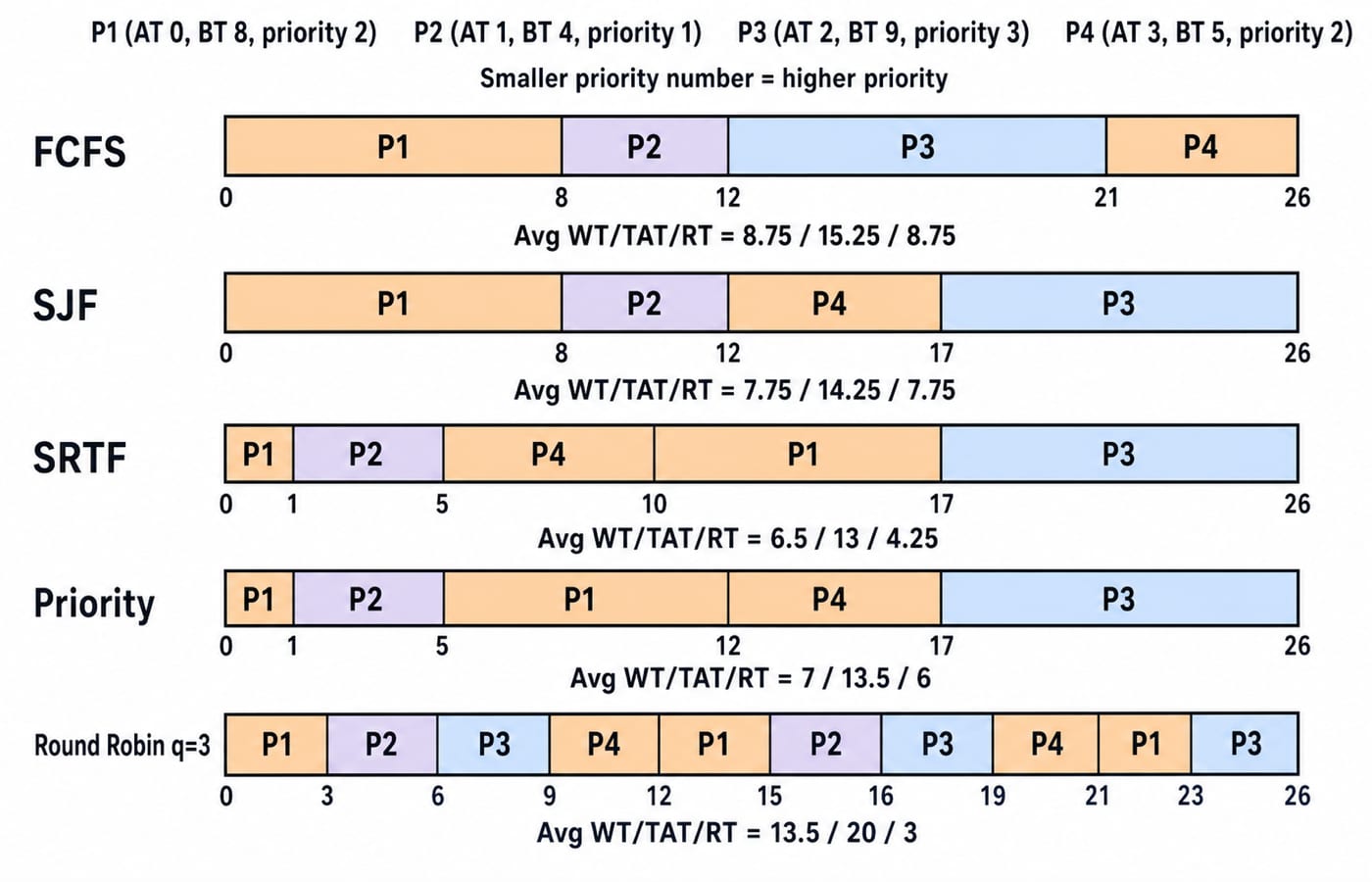
FCFS gives average TAT=61/4=15.25 and WT=RT=35/4=8.75; P4 waits 21-3=18, showing the convoy effect. Non-preemptive SJF gives TAT=(8+11+24+14)/4=14.25 and WT=RT=(0+7+15+9)/4=7.75. P1 must run first because it alone is ready at 0.
For SRTF, P1 has 7 units left when P2 arrives at 1. P2 remains shortest with 3 left at 2 and 2 at 3. Its average TAT=52/4=13, WT=26/4=6.5, and RT=17/4=4.25. Recalculate remaining time at every arrival.
Priority scheduling and Round Robin with switching cost
P2 arrives at 1 and preempts P1. After P2, earlier-arriving P1 wins its tie with P4. Trace: P1 0-1 | P2 1-5 | P1 5-12 | P4 12-17 | P3 17-26. In process order, CT=(12,5,26,17), TAT=(12,4,24,14), WT=(4,0,15,9), RT=(0,0,15,9); averages are 13.5, 7, 6. If ageing improves priority 6 by one every 5 ms, it reaches 3 after 15 ms.
For Round Robin with q=3, boundary arrivals enter before the expired process. Trace: P1 0-3 | P2 3-6 | P3 6-9 | P4 9-12 | P1 12-15 | P2 15-16 | P3 16-19 | P4 19-21 | P1 21-23 | P3 23-26. Then CT=(23,16,26,21), TAT=(23,15,24,18), WT=(15,11,15,13), RT=(0,2,4,6); averages are 20, 13.5, 3. Best response here does not mean best turnaround.
Ten segments create nine inter-process switches. At 0.2 units each, fixed-order elapsed time is 26 + 9(0.2) = 27.8; utilisation is 26/27.8, about 93.5%; throughput is 4/27.8, about 0.144. Do not invent initial or final switch costs.
CPU scheduling algorithms compared
Policy | Decision rule | Strength | Failure mode |
|---|---|---|---|
FCFS | Earliest arrival | Simple | Convoy effect |
SJF | Smallest next burst | Low average waiting for a fixed available set with known bursts | Long-job starvation |
SRTF | Smallest remaining time | Reacts to short arrivals | More preemptions |
Priority | Highest-ranked ready process | Expresses urgency | Starvation without ageing |
Round Robin | Rotate a finite quantum | Quick response | High overhead with tiny quanta |
No policy wins every workload and metric. HRRN maximises (waiting+burst)/burst: A with waiting 6, burst 4 scores 10/4=2.5; B with waiting 6, burst 9 scores 15/9, about 1.67. A wins. LJF chooses the largest burst; LRTF is its preemptive form, opposite to SJF and SRTF.
Traps include ignoring later arrivals, using original instead of remaining time in SRTF, omitting initial idle time, changing tie rules, recomputing response after preemption, subtracting burst twice, and inventing switch cost. After reproducing these traces, CPU scheduling algorithms: FCFS, SJF, Round Robin and priority explained works a simpler set in which all four processes arrive at time zero.
Multilevel queues, MLFQ and advanced scheduling
A Multilevel Queue fixes each process in a queue and defines policies between and within queues. MLFQ lets work move: interactive jobs remain high, jobs consuming a whole quantum drop, and priority boosts limit starvation.
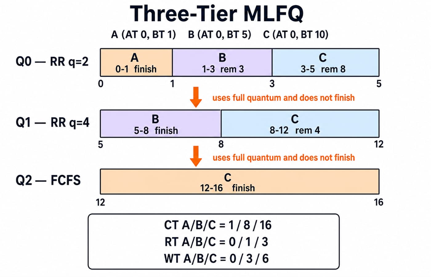
Let A(BT 1), B(BT 5), C(BT 10) arrive at 0. Q0 is RR q=2, Q1 is RR q=4, Q2 is FCFS. Trace: Q0: A 0-1 completes, B 1-3 leaves 3, C 3-5 leaves 8; Q1: B 5-8 completes, C 8-12 leaves 4; Q2: C 12-16 completes. Hence CT = 1, 8, 16, RT = 0, 1, 3, WT = 0, 3, 6. This assumes simultaneous arrivals and no high-queue interruption.
On multiprocessors, load balancing spreads work while affinity preserves cache locality. Real-time scheduling targets deadlines: Rate Monotonic fixes priority by period; EDF chooses the nearest absolute deadline. At 0, EDF selects J1(execution 1, deadline 4) before J2(execution 2, deadline 7).
CPU scheduling numericals and interview questions
For numericals, show the ready queue at each decision, draw the chart, then derive CT, TAT, WT, RT. Variants change preemption, quantum, switch cost, ties or ageing. Diagnose convoy effect, starvation and unfairness from the trace.
Interviews return to four questions. A tiny quantum improves response because every process reaches the CPU sooner, but each slice ends in a context switch: at the 0.2-unit cost used earlier, ten segments already burn 1.8 units of pure overhead, and q=1 would burn far more. SJF predicts the next burst because the real one is unknown at decision time, so exponential averaging carries recent history forward. Starvation is indefinite postponement while the CPU still does useful work, whereas deadlock is a circular wait in which nobody progresses at all. Affinity conflicts with load balancing when migrating a process to an idle core throws away its warm cache, which is why schedulers migrate reluctantly. Name the workload and metric, not a universal winner.
KnowledgeGate carries over 280 CPU scheduling questions, enough to meet every arrival, preemption and tie-break variant more than once. Attempt Process Scheduling MCQs: 12 Solved GATE Questions, then use GATE CS Exam Preparation for the wider line-up.
CPU scheduling: the short version and next step
Use six steps: list arrivals and bursts; mark decisions; update remaining time; read completion from the chart; calculate turnaround, waiting and response; compare with the workload goal and switching cost.
Paper check: average waiting is FCFS 8.75, SJF 7.75, SRTF 6.5, Priority 7, RR 13.5. RR also has response 3 and ten segments. If a value does not follow, redraw the queue.
For sequenced Operating Systems study, use GATE Guidance by Sanchit Sir; for broader timed practice, use the GATE Test Series. If you only need scheduling, reproduce the charts unaided, then use the recap and solved MCQs.
Keep learning
Paging and TLB Explained: Address Translation, EMAT and Exam Traps
Follow one virtual address from its VPN through the TLB to a physical frame, then calculate page-table size, TLB reach and effective memory access time.
Updated 4 Oct 20266 min readOperating Systems
Operating System Scenarios: Solve Scheduling, Concurrency, and Page Replacement
Learn one state-trace method for three common OS problem families, then apply it to complete Round Robin, concurrency, FIFO, and LRU examples.
Updated 29 Sep 20265 min readOperating Systems

Tower Research Hiring Process: Stage-by-Stage Prep for Quant and Dev Roles
Prepare for a Tower Research application without treating one online account as a universal process. Use this role-led map, worked drills, and seven-day plan.
Updated 25 Sep 20265 min readOperating Systems

Capital One Recruitment Process: Stage-by-Stage Guide for India Applicants
Prepare for a Capital One India application with a cautious five-stage map, worked technical and case drills, and a practical 14-hour schedule.
Updated 24 Sep 20265 min readOperating Systems