

FCFS Scheduling: Gantt Charts, Waiting Time and Exam Traps
Learn FCFS scheduling through a four-process trace, a complete metric table, convoy-effect reasoning, and checks for idle time, ties and context switches.
KnowledgeGate Team
Exam prep & CS education
Updated 2 Nov 20265 min read
FCFS sounds like “run the first process first”, yet that shortcut causes mistakes. The real difficulty is preserving ready-queue order when arrival times differ, drawing idle intervals, and keeping completion, turnaround, waiting and response time separate. Calculate every metric from arrivals in one exact four-process trace, then use the same method for the convoy effect, tie rules, context-switch cost and exam-style questions. For the wider comparison, see CPU scheduling algorithms.
FCFS scheduling starts with ready-queue order
First Come, First Served is non-preemptive. When the CPU is free, it selects the ready-queue head, which then runs until its single burst finishes.
Rules:
Enqueue processes by arrival time.
Preserve the stated input or enqueue order for equal arrivals.
Whenever the CPU becomes free, run the process at the queue head.
Arrival order is not process-ID or shortest-burst order. A new arrival joins the tail without displacing the running process. Without a stated equal-arrival tie rule, the order is underdetermined.
FCFS normally avoids starvation with finite work ahead, but mean waiting is order-sensitive. A long job delaying short jobs creates the convoy effect. FIFO page replacement and FCFS disk scheduling apply queues to different state.
Build the FCFS Gantt chart before calculating any average
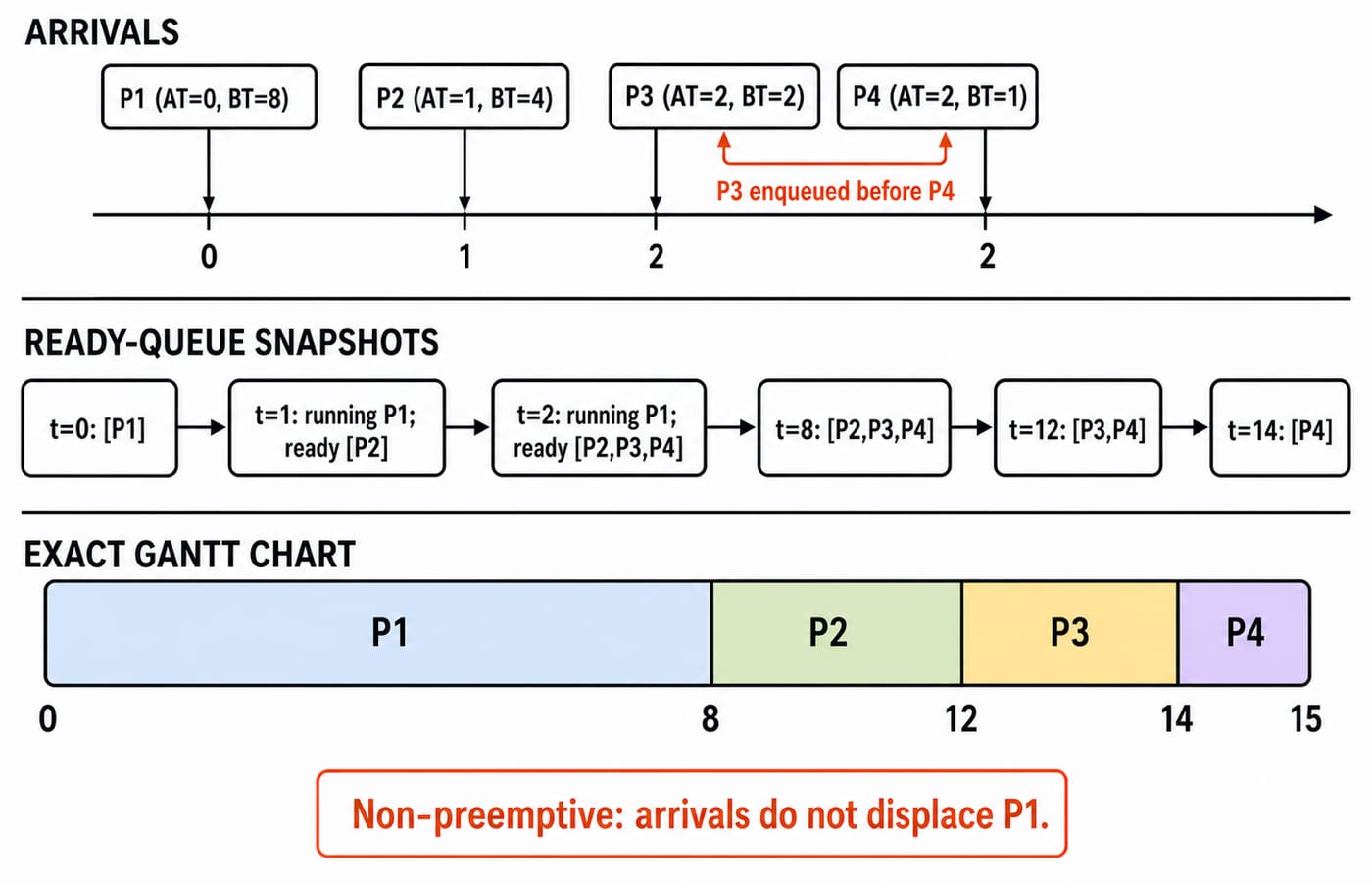
Burst means required CPU time, not finishing time. P3 is enqueued before P4 at time 2.
Process | Arrival time | Burst time | Same-arrival enqueue order |
|---|---|---|---|
P1 | 0 | 8 | first |
P2 | 1 | 4 | second |
P3 | 2 | 2 | third |
P4 | 2 | 1 | fourth |
At t=0, P1 starts. P2 joins at t=1. At t=2, P3 then P4 join, giving [P2, P3, P4]; P1 continues. Select P2 at t=8, P3 at t=12 and P4 at t=14.
Chart: 0 | P1 | 8 | P2 | 12 | P3 | 14 | P4 | 15. Segment lengths 8, 4, 2, 1 match the bursts; busy time is 8 + 4 + 2 + 1 = 15. The queue stays non-empty, so there is no idle gap.
Calculate completion, turnaround, waiting and response time
Start time ST is first execution; completion CT is the segment's right edge. For arrival AT and burst BT:
Turnaround time:
TAT = CT - ATWaiting time:
WT = TAT - BTResponse time:
RT = ST - AT
Here RT = WT because each process has one non-preemptive burst, not as a universal identity.
Process | ST | CT | TAT | WT | RT |
|---|---|---|---|---|---|
P1 | 0 | 8 |
|
|
|
P2 | 8 | 12 |
|
|
|
P3 | 12 | 14 |
|
|
|
P4 | 14 | 15 |
|
|
|
Totals are 8+11+12+13=44 for TAT and 0+7+10+12=29 for WT. Therefore average TAT is 44/4=11; average WT and RT are 29/4=7.25. Without context-switch overhead, utilisation is 15/15 × 100 = 100%, and throughput is 4/15, about 0.267 processes per time unit. Checksum: sum(TAT) = sum(WT) + sum(BT), so 44 = 29 + 15.
See the convoy effect in the same four processes
P1 runs from 0 to 8. P2 arrives at 1 and waits 7 units. P3 and P4 arrive at 2, but start at 12 and 14. Arrival fairness does not minimise mean waiting.
For comparison only, choose the shortest ready job after P1. The order is P4 8-9 | P3 9-11 | P2 11-15. Waiting is P4 8-2=6, P3 9-2=7, P2 11-1=10, and P1 0; mean WT is (0+6+7+10)/4 = 5.75, versus FCFS 7.25. This does not prove one algorithm best for every workload.
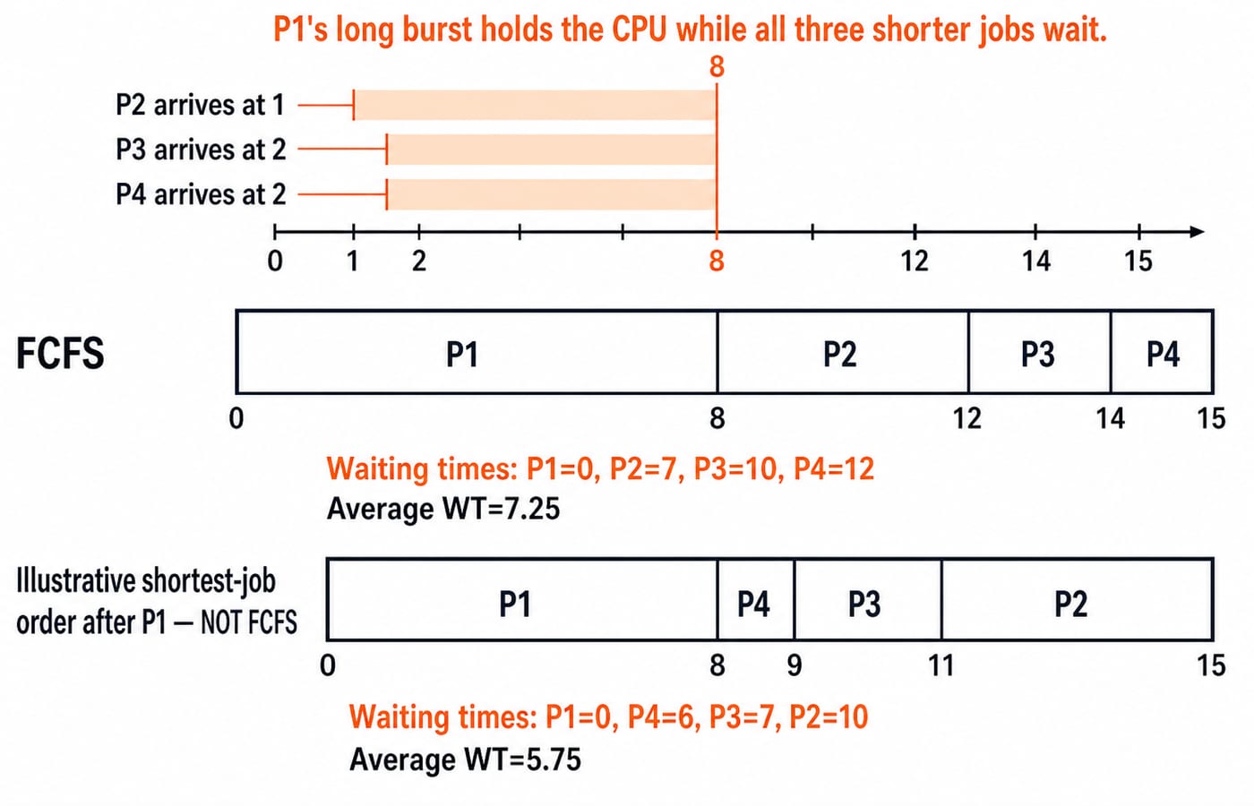
FCFS has simple, predictable queue discipline and needs no burst estimate. Its costs are order-sensitive waiting and no response guarantee for short jobs. P3 and P4 are delayed, not starved, because both run.
Handle idle time, equal arrivals and context-switch cost explicitly
For A(AT=2,BT=3) and B(AT=7,BT=2), draw Idle 0-2 | A 2-5 | Idle 5-7 | B 7-9. WT values are 0; TAT values are 3 and 2. Over t=0 to t=9, busy time is 5, utilisation is 5/9 × 100 = 55.56%, and throughput is 2/9. Do not shift A to zero or stretch its burst across idle time.
For X(AT=4,BT=2) and Y(AT=4,BT=3), stated order X then Y gives Idle 0-4 | X 4-6 | Y 6-9. Without a tie convention, both orders are valid FCFS outcomes. Sorting by burst changes the policy.
Charge a 1-unit switch between main-example processes, not after the last. The order is unchanged: P1 0-8 | CS 8-9 | P2 9-13 | CS 13-14 | P3 14-16 | CS 16-17 | P4 17-18. Waiting times are 0, 8, 12, 15; average WT is 35/4=8.75. State the convention because overhead may be excluded or placed differently.
How exam-style questions test FCFS scheduling
Exam-style families cover charts, averages, missing values, ties, idle or switch intervals, comparisons, convoy effect, starvation, preemption and response. For a named examination, confirm the current syllabus and paper pattern on its official site.
Use this order every time:
Copy the process table and establish stable arrival-plus-tie order.
Set a time cursor. If the queue is empty, advance it and draw
Idle.Otherwise dispatch the queue head and mark its start and completion.
Calculate every row from the formulas, then average.
Check
segment length = burst,CT >= AT, andsum(TAT) = sum(WT) + sum(BT)for a single-burst table.
Then use Process Scheduling MCQs for adjacent practice across scheduling concepts.
Avoid the FCFS mistakes that change the entire answer
Sort by burst time-> that is an SJF-style choice, not FCFS.Preempt P1 when P2 arrives at t=1-> FCFS is non-preemptive here.Put P4 before P3 because its burst is 1-> the stated tie order is P3 then P4.Start the first process at zero regardless of arrival-> draw Idle until its arrival.P2 waiting time = CT-AT = 11->11is TAT; WT is11-4=7.P4 response time = CT-AT = 13-> RT isST-AT = 14-2=12.Average waiting = average completion minus average burst-> arrivals break this shortcut; calculate each TAT.FCFS always has the highest waiting time-> one workload proves no universal ranking.A long wait means starvation-> P4 waits12units but runs.Always add context switches-> add them only when a cost and convention are specified.CPU utilisation is automatically 100%-> the idle example gives55.56%over its stated window.
FCFS scheduling: the short version and next step
Method: preserve queue order -> draw busy and idle intervals -> read ST and CT -> calculate TAT, WT and RT per row -> average -> check. Main answer: P1,P2,P3,P4, boundaries 0-8-12-14-15, average TAT 11, average WT and RT 7.25, utilisation 100% without overhead.
Self-check: keep P1 and P2, but enqueue P4 before P3 at t=2. Chart: P1 0-8 | P2 8-12 | P4 12-13 | P3 13-15. WT values are P1=0, P2=7, P4=10, P3=11, so average WT is 28/4=7. TAT totals 43, average TAT is 10.75, and 43=28+15.
Continue with Operating Systems for GATE or the CS Fundamentals hub. For structured study, ZERO TO HERO is an optional core-CS course.
Go deeper with the full courseOperating System
Keep learning

Round Robin Scheduling Explained: Gantt Charts, Waiting Time and GATE Traps
Learn a fixed Round Robin queue convention, trace staggered arrivals, calculate CT, TAT, WT and RT, and see how quantum size and context-switch cost change results.
Updated 9 Oct 20265 min read128 viewsOperating Systems
SJF and SRTF Scheduling: Concepts, Gantt Charts and Worked Examples
Learn how non-preemptive SJF and preemptive SRTF schedule the same four processes, then calculate CT, TAT and WT while avoiding arrival, tie and Gantt-chart traps.
Updated 8 Nov 20265 min readOperating Systems

LJF and HRRN CPU Scheduling: Worked Gantt Charts, Formula and Exam Traps
Solve one five-process data set under non-preemptive LJF and HRRN, then compare every completion, turnaround, and waiting time.
Updated 4 Nov 20266 min readOperating Systems

CPU Scheduling in Operating Systems: Algorithms, Gantt Charts and Worked Examples
Trace one process set through five CPU scheduling policies, calculate every core metric, and extend the method to switching costs and MLFQ.
Updated 17 Aug 20266 min read66 viewsOperating Systems