

Multilevel Queue Scheduling: Concepts, Worked Examples and GATE Exam Patterns
Learn to separate queue selection from local scheduling, trace MLQ and MLFQ examples, calculate waiting time correctly, and spot rule changes that alter the chart.
KnowledgeGate Team
Exam prep & CS education
Updated 5 Nov 20266 min read

A multilevel-queue problem can look like an ordinary Gantt-chart question until one process follows Round Robin, another follows FCFS, and a rule between queues decides which may run. A correct trace fixes process classification, inter-queue selection and intra-queue scheduling before any arithmetic. Those choices determine whether an arrival preempts the runner and whether a process may move. Use the CS Fundamentals for Exams & Placements when you want to connect scheduling with the rest of core computer science.
Multilevel queue scheduling: separate classification from scheduling
Multilevel queue scheduling, or MLQ, divides ready processes into fixed classes. For example, Q0 = system, Q1 = interactive, and Q2 = batch. The labels may change, but membership stays fixed unless the question permits movement.
The inter-queue scheduler chooses a queue, perhaps by strict priority Q0 > Q1 > Q2. The intra-queue scheduler chooses within it, perhaps RR with 2 ms quantum in Q0, RR with 4 ms in Q1, and FCFS in Q2. For a single ready queue, CPU scheduling: FCFS, SJF, Round Robin and priority. MLQ first chooses a queue, while MLFQ may also move work between queues.
Decision | Question to ask | Example |
|---|---|---|
Classification | Which queue owns the process? |
|
Inter-queue policy | Which non-empty queue gets the CPU? |
|
Intra-queue policy | Which process within that queue runs? |
|
Movement | Can a process change queue? | No in this MLQ model |
Priority-number conventions vary, so follow the written ordering.
Multilevel queue worked example: trace strict priority first
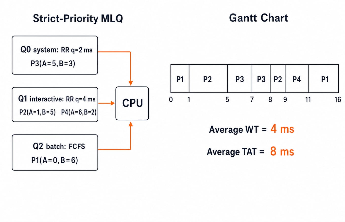
Use one CPU, zero context-switch cost, and strict preemptive priority Q0 > Q1 > Q2. Q0 uses RR with q0 = 2 ms, Q1 uses RR with q1 = 4 ms, and Q2 uses FCFS. A newly non-empty higher queue preempts immediately. An expired RR job joins its queue's tail. Process simultaneous boundary events before dispatch. Processes never change queues.
Process | Queue | Arrival | Burst |
|---|---|---|---|
P1 | Q2 | 0 | 6 ms |
P2 | Q1 | 1 | 5 ms |
P3 | Q0 | 5 | 3 ms |
P4 | Q1 | 6 | 2 ms |
At each event, show remaining time in brackets:
Time | Ready state after the event | Dispatch |
|---|---|---|
0 | Q2: P1(6) | P1 |
1 | Q1: P2(5); Q2: P1(5) | P2 preempts P1 |
5 | Q0: P3(3); Q1: P2(1); Q2: P1(5) | P3; P2 was requeued |
6 | Q0: P3(2); Q1: P2(1), P4(2); Q2: P1(5) | P3 continues |
7 | Q0: P3(1); Q1: P2(1), P4(2); Q2: P1(5) | P3 is requeued, then redispatched |
8 | Q1: P2(1), P4(2); Q2: P1(5) | P2 |
9 | Q1: P4(2); Q2: P1(5) | P4 |
11 | Q2: P1(5) | P1 |
16 | All queues empty | Stop |
The chart is 0 | P1 | 1 | P2 | 5 | P3 | 7 | P3 | 8 | P2 | 9 | P4 | 11 | P1 | 16. Adjacent P3 segments stay separate because t=7 records quantum expiry and redispatch.
Process | Completion C | Turnaround C - A | Waiting TAT - burst |
|---|---|---|---|
P1 | 16 | 16 | 10 |
P2 | 9 | 8 | 3 |
P3 | 8 | 3 | 0 |
P4 | 11 | 5 | 3 |
Average turnaround is (16 + 8 + 3 + 5) / 4 = 32 / 4 = 8 ms. Average waiting is (10 + 3 + 0 + 3) / 4 = 16 / 4 = 4 ms. Also, 6 + 5 + 3 + 2 = 16 ms, matching the busy timeline.
Inter-queue policies: strict priority, CPU shares and starvation
With strict priority, a lower queue runs only when every higher queue is empty. P1 waits from t=1 to t=11, totalling 10 ms. Continued higher-priority arrivals can leave Q2 waiting without a finite bound. That risk is starvation, but it does not arise in every MLQ system.
For a CPU-share alternative, let each 20 ms cycle run Q0 for 10 ms (50%), Q1 for 6 ms (30%), then Q2 for 4 ms (20%). If all queues stay non-empty, a Q2 job ready at t=0 and needing 12 ms runs at 16-20, 36-40, and 56-60. It completes at t=60; waiting is 60 - 12 = 48 ms. Slot order and unused-share redistribution must be stated.
Aging raises waiting work's effective priority, a reserved share guarantees service, and a periodic boost may reset feedback levels. None is automatically part of fixed MLQ.
Multilevel feedback queue: movement changes the algorithm
Property | MLQ | MLFQ |
|---|---|---|
Meaning of queue | Fixed process class | Changing scheduling state |
Movement | Normally absent | Promotion or demotion under stated rules |
Local policies | May differ by queue | May differ by queue |
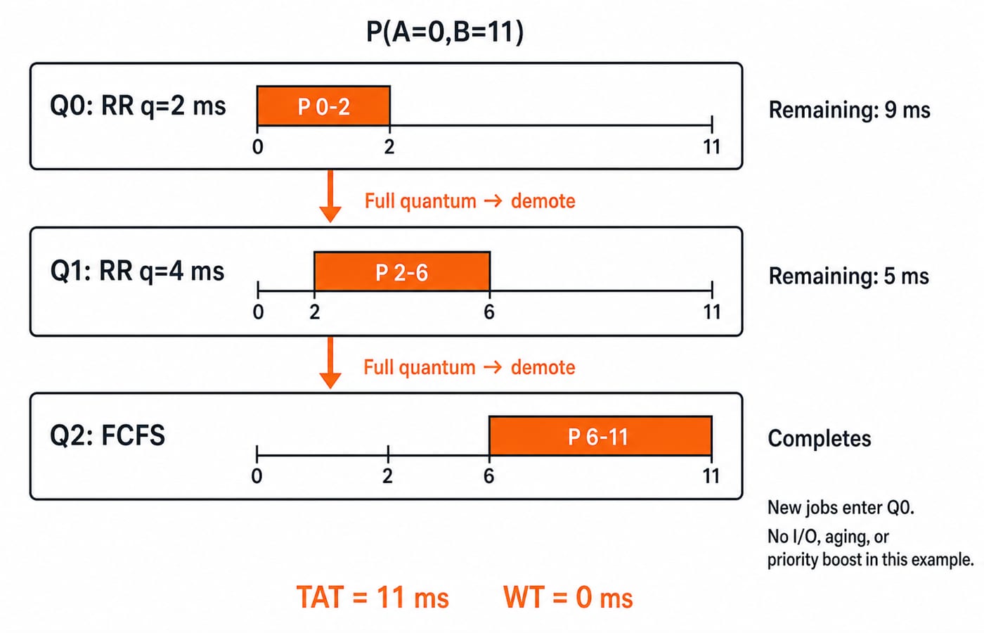
For an exact MLFQ trace, Q0 uses RR 2 ms, Q1 uses RR 4 ms, and Q2 uses FCFS. New work enters Q0; using a full quantum without finishing causes one-level demotion. There is no I/O, aging, periodic boost, or context-switch cost.
Process P arrives at t=0 with burst 11 ms. It runs in Q0 from 0-2, leaves 9 ms, then runs in Q1 from 2-6, leaving 5 ms. It finishes in Q2 from 6-11. Thus TAT = 11 - 0 = 11 ms and WT = 11 - 11 = 0 ms because no competitor exists.
A process finishing in its first 2 ms slice never reaches Q1. A process blocking early for I/O needs a stated retain-or-promote rule before its next queue is known.
Multilevel queue traps: one rule can change the chart
Change only the inter-queue rule: priority is non-preemptive at process level, so the running process finishes before a higher queue takes over. The chart becomes P1 0-6 | P3 6-8 | P3 8-9 | P2 9-13 | P4 13-15 | P2 15-16.
P1 to P4 complete at 6, 16, 9, 15. Their waiting times are 0, 10, 1, 7; the average is (0 + 10 + 1 + 7) / 4 = 18 / 4 = 4.5 ms. "Priority queues" alone does not establish preemption.
Other wrong moves and corrections are:
RR across all processes: choose a queue first, then apply its local rule.
Move a long Q1 job to Q2: movement needs MLFQ or an explicit rule.
Count only the last pause: use
WT = completion - arrival - total burst.Run P4 before P2 at
t=8: preserve RR tail order.Merge P3's slices: retain decision boundaries after redispatch.
Add aging: use it only when specified.
Write this assumption box first:
Queue assignment: Which process belongs where?
Inter-queue rule: Which queue wins?
Intra-queue rule: Which local algorithm applies?
Preemption rule: Can an arrival interrupt running work?
Movement or aging rule: Can membership or effective priority change?
State any missing interpretation before calculating.
Multilevel queue exam patterns: recognise, trace and calculate
Common forms ask you to identify MLQ versus MLFQ, select from non-empty queues, build a chart, calculate completion, turnaround, waiting or response time, diagnose starvation, compare policies, or judge statements about membership and feedback. These are problem forms, not an official distribution.
Use this solving order:
Draw one row per queue; record queue, arrival, and burst.
Write the inter-queue policy above and local policies beside the rows.
Advance to the next arrival, quantum expiry, completion, or stated boost.
Update remaining bursts and queue order.
Calculate from the completed chart, then use Process Scheduling MCQs: 12 Solved (GATE) for trace practice.
Closed-book answers: the strict-preemptive chart ends at 16 ms, P1 waits 10 ms, average waiting is 4 ms, and average turnaround is 8 ms. The non-preemptive average is 4.5 ms. The feedback job follows Q0 -> Q1 -> Q2 at 0-2, 2-6, and 6-11.
Multilevel queue scheduling: the short version and next step
Remember classify -> choose a queue -> schedule within that queue -> update events -> calculate metrics. MLQ fixes membership; MLFQ changes it under stated feedback rules. Redraw the first example, alter only preemption, and explain the new order.
Self-check: make P3's burst 2 ms. It finishes at t=7; P2 runs 7-8, P4 8-10, and P1 10-15. The chart is P1 0-1 | P2 1-5 | P3 5-7 | P2 7-8 | P4 8-10 | P1 10-15.
For organised preparation, GATE Guidance by Sanchit Sir is an optional structured route. For this concept alone, redo both traces and use the scheduling comparison and practice set above.
Go deeper with the full courseOperating System
Keep learning

Multilevel Queue Scheduling MCQs: 10 Solved Questions with Explanations
Attempt 10 published objective questions on MLFQ behaviour, scheduler matching, two-level scheduling and weighted completion time. Each answer explains the decisive rule.
Updated 30 Oct 20268 min read91 viewsOperating System MCQs
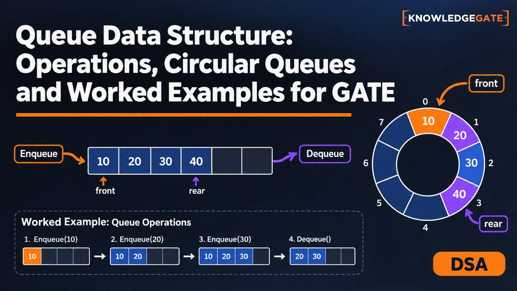
Queue Data Structure: Operations, Circular Queues and Worked Examples for GATE
Learn queue operations through a five-slot circular queue trace, then connect the same FIFO rule to linked lists, BFS and the two-stack implementation.
Updated 4 Oct 20266 min read103 viewsDSA & Algorithms

Priority Queue MCQs: 12 Solved Questions on Heaps, Deques and Variants
Attempt 12 verified priority queue and queue-variant MCQs, then learn from concise heap, array, circular queue and deque traces.
Updated 25 Sep 20267 min readData Structures MCQs
Circular Queue and Deque for GATE: The Full-Empty Condition Settled with a Worked Trace
Trace a size-5 circular queue through enqueue, dequeue, wraparound and rejection, then separate its pointer rules from the operations of a deque.
Updated 9 Sep 20266 min read54 viewsDSA & Algorithms