

SJF and SRTF Scheduling: Concepts, Gantt Charts and Worked Examples
Learn how non-preemptive SJF and preemptive SRTF schedule the same four processes, then calculate CT, TAT and WT while avoiding arrival, tie and Gantt-chart traps.
KnowledgeGate Team
Exam prep & CS education
Updated 8 Nov 20265 min read
SJF and SRTF both favour short CPU work, but they behave differently when a shorter process arrives after another has started. That single distinction can change every completion, turnaround and waiting-time answer. The same four-process dataset yields two complete Gantt charts and exact completion, turnaround and waiting-time calculations under both policies. Correct arrival and tie rules prevent most wrong answers. All times below are illustrative time units.
SJF and SRTF: the one distinction that changes the schedule
A single CPU selects only from the ready queue. Arrival time (AT) is when a process becomes ready, burst time (BT) is its required CPU work, and remaining time (RT) is unfinished work. A future arrival is ineligible.
Non-preemptive Shortest Job First, or SJF, chooses the smallest ready burst whenever the CPU becomes free, then lets it finish. Shortest Remaining Time First, or SRTF, reconsiders at each arrival or completion and preempts for a strictly smaller RT.
Comparison | SJF | SRTF |
|---|---|---|
Selection key | BT of waiting jobs | RT of ready jobs |
Decision points | CPU becomes free | Arrival or completion |
Can a new arrival preempt? | No | Yes, if RT is smaller |
Value that changes while running | None used for reselection | RT |
Main calculation risk | Using future arrivals | Mishandling split segments |
For the arrival-order baseline and convoy effect on nearly the same burst set, see FCFS Scheduling: Gantt Charts, Waiting Time and Exam Traps. This analysis instead isolates non-preemptive SJF choices and SRTF preemption at arrival boundaries.
Set the rules and formulas before drawing either Gantt chart
Use this common dataset and preserve its process order:
Process | Arrival time | Burst time |
|---|---|---|
P1 | 0 | 8 |
P2 | 1 | 4 |
P3 | 2 | 2 |
P4 | 4 | 1 |
Assume one CPU, no I/O blocking, zero context-switch overhead, supplied bursts and work-conserving scheduling. Total work is 8 + 4 + 2 + 1 = 15, so this no-idle chart must end at 15.
Fix ties first. Preempt only for a strictly smaller RT; equality keeps the running process. At a fresh dispatch, choose earlier arrival, then lower process number. A stated rule overrides this one.
Use TAT = CT - AT and WT = TAT - BT. Completion time (CT) is the final segment's right endpoint. Calculate all rows before averaging. If nobody is ready, draw Idle until the next arrival.
Worked example 1: non-preemptive SJF
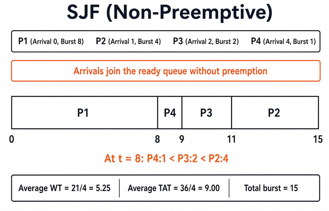
At t=0, only P1 is ready, so it runs 0 to 8; SJF cannot wait for future short jobs. P2, P3 and P4 arrive while P1 runs but cannot preempt. At 8, their waiting bursts order as P4 1, P3 2, P2 4.
Gantt chart: 0 | P1 | 8 | P4 | 9 | P3 | 11 | P2 | 15
Process | CT | TAT = CT - AT | WT = TAT - BT |
|---|---|---|---|
P1 | 8 |
|
|
P2 | 15 |
|
|
P3 | 11 |
|
|
P4 | 9 |
|
|
Total TAT is 8 + 14 + 9 + 5 = 36, averaging 9.00. Total WT is 0 + 10 + 7 + 4 = 21, averaging 5.25. Segments total 8 + 1 + 2 + 4 = 15.
Worked example 2: solve SRTF on the same processes
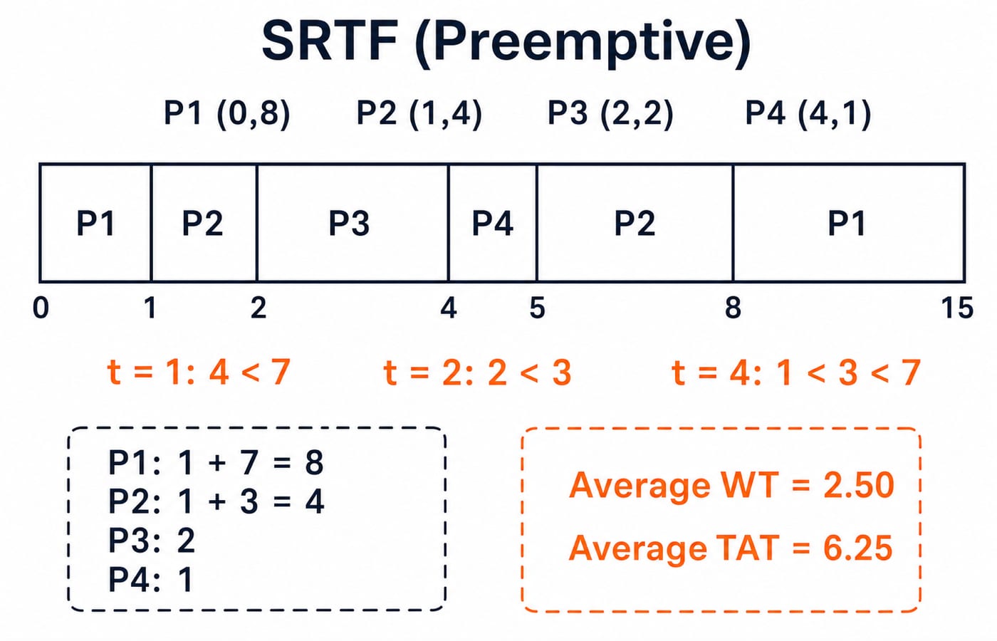
P1 runs 0 to 1, leaving 7. P2 arrives with 4, so 4 < 7 preempts P1. P2 runs to 2, leaving 3; P3 arrives with 2, so 2 < 3 preempts P2. P3 completes at 4, exactly when P4 arrives.
At 4, P4 1 beats P2 RT 3 and P1 RT 7. Run P4 to 5, P2 to 8, then P1 to 15.
Gantt chart: 0 | P1 | 1 | P2 | 2 | P3 | 4 | P4 | 5 | P2 | 8 | P1 | 15
Process | CT | TAT = CT - AT | WT = TAT - BT |
|---|---|---|---|
P1 | 15 |
|
|
P2 | 8 |
|
|
P3 | 4 |
|
|
P4 | 5 |
|
|
Total TAT is 15 + 7 + 2 + 1 = 25, averaging 6.25. Total WT is 7 + 3 + 0 + 0 = 10, averaging 2.50. Split-burst check: P1 1 + 7 = 8, P2 1 + 3 = 4, P3 2, P4 1, total 15.
Compare the two results without overgeneralising
Here SRTF changes average WT from 5.25 to 2.50 and average TAT from 9.00 to 6.25, differences of 2.75. These are dataset-specific, not universal improvements.
P1 shows the fairness cost. SJF gives it WT=0, TAT=8; SRTF interrupts it twice and gives WT=7, TAT=15. P3 and P4 instead wait zero under SRTF. Better averages do not help every process.
SRTF tracks RT and may preempt more. Both policies can delay long jobs while shorter ones keep arriving. If switching cost is supplied, insert it by the stated convention and recompute the timeline.
Fix the traps that produce a plausible but wrong answer
Trap | Why it fails | Correction |
|---|---|---|
Choose P4 first | It arrives at | Start P1 at |
Preempt P1 in SJF | Policy is non-preemptive | Finish P1 at |
Reuse P2 BT | P2 already ran | Use RT |
Set TAT to CT | This ignores AT | Use |
First segment end is CT | Process is unfinished | Use its final endpoint |
Draw Idle only when the queue is empty. Check each boundary and the burst sum: 1+1+2+1+3+7=15.
Separate the initial dispatch, five process-to-process handoffs, and two preemptions at 1 and 2. Context-switch counting follows the question. Equal RT 1 keeps the current process under our tie rule.
How exam-style questions test SJF and SRTF
Questions ask for charts, WT and TAT calculations, preemption counts, or statements about starvation, idle time and ties.
Rapid checks: SJF selects P1 at 0 because it alone is ready. SRTF selects P2 at 1 because 4<7, then P3 at 2 because 2<3. P1 has the largest WT increase, 0 to 7.
Change only P4's arrival to 3. P3 then has RT 1, tying P4's BT 1, so our rule keeps P3 until 4. Another stated tie rule may differ. Next, try the Process Scheduling MCQs.
SJF and SRTF: the short version and next step
Recall:
Build the ready queue from AT.
Use BT for SJF and RT for SRTF.
Apply the stated preemption and tie rule.
Read CT from the final segment.
Calculate
TAT=CT-AT, thenWT=TAT-BT.
Here SJF averages are WT 5.25, TAT 9.00; SRTF averages are WT 2.50, TAT 6.25.
Hide both tables and redraw P1(0,8), P2(1,4), P3(2,2), P4(4,1). Rebuild eight rows, verify burst 15, then explain why SJF keeps P1 while SRTF may interrupt it.
Placement learners can continue with Computer Science Fundamentals for Placements by Sanchit Sir, whose catalog includes Operating Systems. For a broader core-CS route, see the Zero to Hero Complete CS Course. The CS Fundamentals category is the subject hub.
Go deeper with the full courseOperating System
Keep learning

SJF and SRTF Scheduling MCQs: 11 Solved Questions with Step-by-Step Explanations
Solve 11 SJF and SRTF questions with ready-queue decisions, Gantt traces, waiting-time calculations and checked explanations.
Updated 30 Oct 20267 min read129 viewsOperating System MCQs

LJF and HRRN CPU Scheduling: Worked Gantt Charts, Formula and Exam Traps
Solve one five-process data set under non-preemptive LJF and HRRN, then compare every completion, turnaround, and waiting time.
Updated 4 Nov 20266 min readOperating Systems

FCFS Scheduling: Gantt Charts, Waiting Time and Exam Traps
Learn FCFS scheduling through a four-process trace, a complete metric table, convoy-effect reasoning, and checks for idle time, ties and context switches.
Updated 2 Nov 20265 min readOperating Systems

Round Robin Scheduling Explained: Gantt Charts, Waiting Time and GATE Traps
Learn a fixed Round Robin queue convention, trace staggered arrivals, calculate CT, TAT, WT and RT, and see how quantum size and context-switch cost change results.
Updated 9 Oct 20265 min read128 viewsOperating Systems