Round Robin Scheduling Explained: Gantt Charts, Waiting Time and GATE Traps
Learn a fixed Round Robin queue convention, trace staggered arrivals, calculate CT, TAT, WT and RT, and see how quantum size and context-switch cost change results.
KnowledgeGate Team
Exam prep & CS education
Updated 9 Oct 20265 min read66 views
Round Robin gives every process a turn, but one wrong ready-queue update changes the Gantt chart and every derived metric. CPU scheduling algorithms: FCFS, SJF, Round Robin and priority explained compares those four policies on one all-at-zero workload. Under Round Robin alone, three staggered arrivals expose boundary order, response time and explicit switch cost.
Round Robin scheduling: ready queue, time quantum and pre-emption
Round Robin is a pre-emptive ready-queue algorithm. The head process receives at most one time quantum, q. At slice end, an unfinished process moves to the queue tail; a finished process leaves and the next ready process starts a fresh quantum.
Track arrival time AT, burst time BT, completion time CT, and first start:
TAT = CT - ATWT = TAT - BTRT = first start - AT
Waiting time covers ready periods; response time ends at first dispatch. A smaller q usually improves early response but causes more pre-emptions. If q is at least every remaining burst, ready-queue order behaves like FCFS.
Round Robin ready-queue method: fix the event order before drawing
Apply this sequence: dispatch the queue head; run until completion or quantum expiry; admit arrivals whose time has been reached; append an unfinished runner to the tail; dispatch the next head. If the queue is empty, jump to the next arrival and show the idle interval.
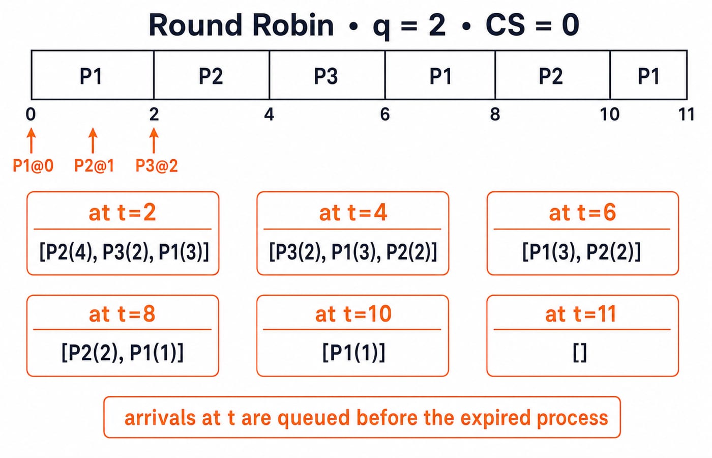
Assume arrivals at time t enter before the process expiring at t is requeued. Equal arrivals use process-label order. Other conventions can produce valid traces, so state the assumption.
Set q=2 and context-switch cost to zero:
Process | AT | BT |
|---|---|---|
P1 | 0 | 5 |
P2 | 1 | 4 |
P3 | 2 | 2 |
Queue entries include remaining burst, such as P1(3) after P1's first slice.
Round Robin worked example: build the Gantt chart step by step
P1 runs from 0-2, leaving P1(3). P2 arrived at t=1, and P3 arrives at t=2, so the declared rule places P3 before requeued P1.
Interval | Result at the interval end | Queue for the next dispatch |
|---|---|---|
| P1 has 3 left |
|
| P2 has 2 left |
|
| P3 finishes |
|
| P1 has 1 left |
|
| P2 finishes |
|
| P1 finishes |
|
Gantt chart: 0 | P1 | 2 | P2 | 4 | P3 | 6 | P1 | 8 | P2 | 10 | P1 | 11.
Two checks: executed CPU time is 5 + 4 + 2 = 11, matching the final clock without idle or overhead. Every slice is at most 2, and no remaining burst becomes negative.
Round Robin waiting time, turnaround time and response time
Process | AT | BT | First start | CT | TAT | WT | RT |
|---|---|---|---|---|---|---|---|
P1 | 0 | 5 | 0 | 11 | 11 | 6 | 0 |
P2 | 1 | 4 | 2 | 10 | 9 | 5 | 1 |
P3 | 2 | 2 | 4 | 6 | 4 | 2 | 2 |
For P2, TAT = 10 - 1 = 9, WT = 9 - 4 = 5, and RT = 2 - 1 = 1. The averages are:
Average TAT:
(11 + 9 + 4) / 3 = 8Average WT:
(6 + 5 + 2) / 3 = 13/3, about4.33Average RT:
(0 + 1 + 2) / 3 = 1
P1 waits from 2-6 for 4 units and from 8-10 for 2, totalling 6. Its response time is zero because first service was immediate.
Round Robin quantum and context-switch cost: what the Gantt chart hides
Compare quantum sizes with all three processes arriving at zero and bursts P1=5, P2=4, P3=2. With q=2: P1 0-2, P2 2-4, P3 4-6, P1 6-8, P2 8-10, P1 10-11. Average response is (0+2+4)/3 = 2; average waiting is (6+6+4)/3 = 16/3, about 5.33.
With q=10, the FCFS-like chart is P1 0-5, P2 5-9, P3 9-11. Average response and waiting are both (0+5+9)/3 = 14/3, about 4.67.
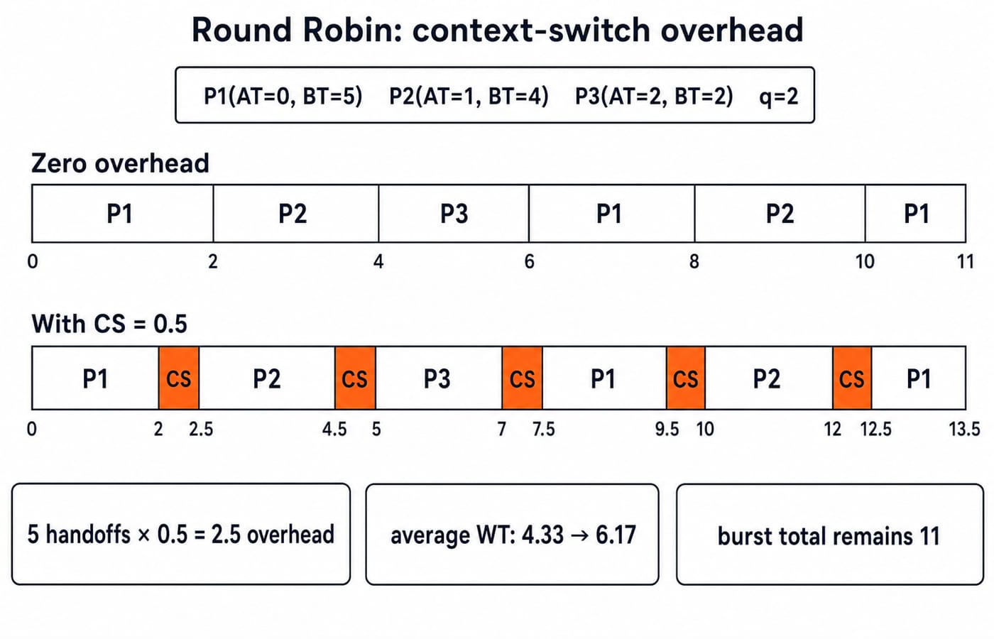
Now charge the staggered-arrival trace 0.5 only for a handoff to a different process, not before the first dispatch or after the last completion. Five handoffs add 2.5, producing P1 0-2, CS 2-2.5, P2 2.5-4.5, CS 4.5-5, P3 5-7, CS 7-7.5, P1 7.5-9.5, CS 9.5-10, P2 10-12, CS 12-12.5, P1 12.5-13.5.
Thus CT=(13.5,12,7), TAT=(13.5,11,5), and WT=(8.5,7,3). Average waiting is 18.5/3, about 6.17. Context-switch time adds to waiting, not CPU burst, so do not subtract it from BT.
Round Robin traps: boundary arrivals, queue resets and metric mix-ups
Trap | Wrong move | Correction |
|---|---|---|
Queue order | Re-sort by arrival after every slice | Keep the FIFO ready queue |
Early finish | Give the next process the unused slice | Start a fresh quantum |
Requeue | Run an unfinished process again immediately | Append it to the tail |
Overhead | Add a switch when cost is zero | Charge only the stated rule |
Waiting | Include CPU execution in WT | Use |
Non-zero arrivals | Use | First compute |
Response | Treat RT as total waiting | Stop RT at first dispatch |
Boundary order can change the answer. If expired P1 is requeued before the t=2 arrival, an alternative is P1 0-2, P2 2-4, P1 4-6, P3 6-8, P2 8-10, P1 10-11. P3 then has CT=8 and WT=8-2-2=4, instead of CT=6 and WT=2. Never mix metrics from the two conventions.
Preserve idle time. For P1(AT=3,BT=2), P2(AT=6,BT=1), and q=2, the chart is Idle 0-3, P1 3-5, Idle 5-6, P2 6-7. A quantum starts on dispatch; idle time belongs to no burst.
Round Robin GATE practice: trace first, calculate second
Use this 30-second method: copy AT and BT; write q and the boundary convention; track a remaining-burst queue; mark completion times; then derive the metrics. Check that final time equals burst total plus idle plus overhead. For q=2 with AT=(0,1,2) and BT=(5,4,2), retrieve CT=(11,10,6), average WT=4.33, and average RT=1.
Operating System Scenarios: Solve Scheduling, Concurrency, and Page Replacement applies the same arrival-before-requeue rule to a compact q=2 workload, then carries its invariant method into race conditions and page replacement. Round Robin-only practice should go further: distinguish RT from WT, recompute the alternative boundary order, and price handoffs only after the zero-overhead chart is stable. Use GATE CS Exam Preparation for subject-wide revision.
Round Robin scheduling: the short version and next step
Remember five points: use a FIFO queue; run for min(q, remaining burst); admit arrivals by the declared boundary rule; requeue only an unfinished process; derive metrics after fixing completion times. WT measures ready-queue delay; RT measures delay to first service.
Redraw the chart, recover CT=(11,10,6), add five 0.5 switches, and prove the clock changes from 11 to 13.5 while burst total stays 11. Continue with GATE Guidance by Sanchit Sir and reproduce the trace and formulas without looking back at the tables.
Keep learning

Critical Section in Process Synchronization: Race Conditions and Correctness Worked Step by Step
See how two sensible updates to x can finish at 6, 7, or 8. The worked trace connects race conditions to mutual exclusion, progress, bounded waiting, and safe synchronization choices.
Updated 21 Oct 20266 min readOperating Systems

System Calls and Dual Mode in OS: Mode-Bit Trace, Worked Example and Exam Traps
Follow one read() call across the user-kernel boundary, calculate its stated overhead, and learn the distinctions that make system-call questions easier.
Updated 17 Oct 20265 min readOperating Systems
Semaphores and Process Ordering in OS: P/V Traces, Worked Examples and GATE Traps
Learn one consistent semaphore convention, then trace ordering constraints, shared-variable updates, bounded-buffer permits, rendezvous, and deadlock step by step.
Updated 13 Oct 20265 min readOperating Systems
Paging and TLB Explained: Address Translation, EMAT and Exam Traps
Follow one virtual address from its VPN through the TLB to a physical frame, then calculate page-table size, TLB reach and effective memory access time.
Updated 4 Oct 20266 min readOperating Systems