

Gradient Boosting Regression: Build Two Residual-Correcting Trees Step by Step
See every stage of gradient boosting regression on five data points, from the initial mean through two residual-fitted stumps and their additive predictions.
KnowledgeGate Team
Exam prep & CS education
Updated 16 Nov 20266 min read

“Each tree fixes the previous tree's mistakes” sounds intuitive, but it hides what becomes the next tree's training label, where the learning rate enters, and how the outputs combine at prediction time. The worked trace uses x = (1,2,3,4,5) and y = (1,2,3,8,12), begins at F_0 = 5.2, and fits two depth-1 trees with eta = 0.5. Training MSE falls from 17.36 to 5.84, then to 2.21.
Gradient boosting is an additive model built in sequence
At stage m, the regression model is
F_m(x) = F_(m-1)(x) + eta T_m(x).
Here, F_(m-1) is the ensemble so far, T_m is the new shallow tree, and eta > 0 scales its correction. Values in (0,1] are commonly used for shrinkage; this trace uses eta = 0.5. A prediction adds the baseline and every shrunken correction, not the latest tree output alone. The Skill Development Courses category provides the broader setting for AI and machine-learning study.
For L_i = (1/2)(y_i - F(x_i))^2, the negative gradient is -partial L_i / partial F(x_i) = y_i - F(x_i) = r_i. This is why squared-error boosting fits residuals. Other differentiable losses use pseudo-residuals, and their optimal leaf updates need not be raw means. Tree m must wait for F_(m-1) to produce its targets, unlike a parallel ensemble. The ML & Data Science hub places this idea in its wider subject area.
Start gradient boosting regression with the best constant prediction
Under squared error, the best constant is the sample mean:
F_0 = (1 + 2 + 3 + 8 + 12) / 5 = 26 / 5 = 5.2.
|
|
|
|
|
|---|---|---|---|---|
1 | 1 | 5.2 | -4.2 | 17.64 |
2 | 2 | 5.2 | -3.2 | 10.24 |
3 | 3 | 5.2 | -2.2 | 4.84 |
4 | 8 | 5.2 | 2.8 | 7.84 |
5 | 12 | 5.2 | 6.8 | 46.24 |
Negative residuals show that the baseline overpredicts the first three targets. Positive residuals show that it underpredicts the last two. The starting MSE is
(17.64 + 10.24 + 4.84 + 7.84 + 46.24) / 5 = 86.80 / 5 = 17.36.
MSE remains the comparison metric even though the gradient derivation uses half squared error. Multiplying the objective by a positive constant does not change its best splits or fitted values.
Fit the first tree to the baseline residuals
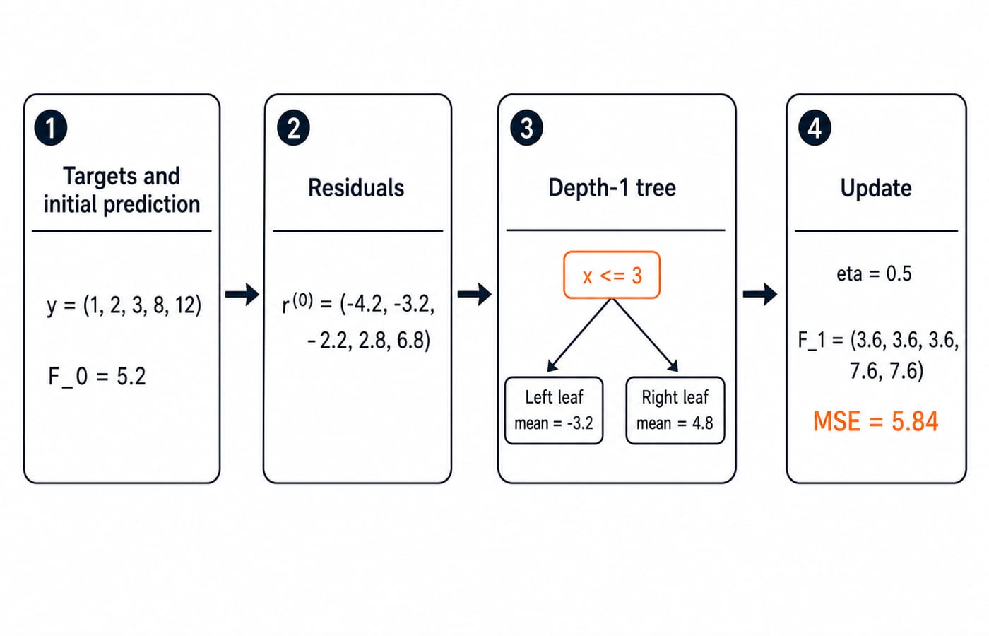
Tree 1 is fitted to (x_i, r_i^(0)), not to the original y_i. Comparing every possible stump split by residual sum of squares gives:
Split after | 1 | 2 | 3 | 4 |
|---|---|---|---|---|
SSE | 64.75 | 41.1667 | 10 | 29 |
The unique minimum is 10, so the split is x <= 3 versus x > 3. Each leaf returns its mean residual:
left = (-4.2 - 3.2 - 2.2) / 3 = -9.6 / 3 = -3.2
right = (2.8 + 6.8) / 2 = 9.6 / 2 = 4.8
Therefore, T_1(x) = -3.2 on the left and T_1(x) = 4.8 on the right. Applying shrinkage,
F_1 = 5.2 + 0.5T_1.
The first three predictions become 5.2 - 1.6 = 3.6; the last two become 5.2 + 2.4 = 7.6. The leaf values -3.2 and 4.8 are corrections, not final target predictions.
Recompute residuals and fit the second correcting tree
Tree 2 needs fresh targets calculated from F_1:
|
|
|
|
|---|---|---|---|
1 | 1 | 3.6 | -2.6 |
2 | 2 | 3.6 | -1.6 |
3 | 3 | 3.6 | -0.6 |
4 | 8 | 7.6 | 0.4 |
5 | 12 | 7.6 | 4.4 |
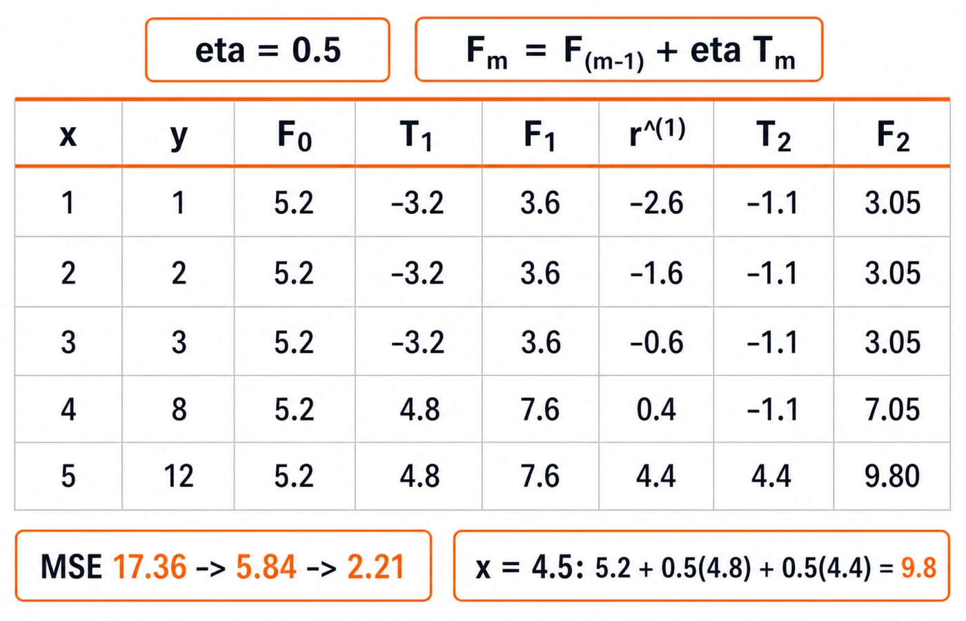
Stage-one MSE is (6.76 + 2.56 + 0.36 + 0.16 + 19.36) / 5 = 29.20 / 5 = 5.84. The split SSE values for r^(1) are 20.75, 14.5, 10, and 5 after x = 1, 2, 3, 4, respectively. Thus tree 2 splits at x <= 4.
Its left output is (-2.6 - 1.6 - 0.6 + 0.4) / 4 = -4.4 / 4 = -1.1; its right output is 4.4. So T_2(x) = -1.1 for x <= 4 and 4.4 otherwise. Adding this correction to F_1, not F_0, gives
F_2 = F_1 + 0.5T_2 = (3.05, 3.05, 3.05, 7.05, 9.80).
The new residuals are (-2.05, -1.05, -0.05, 0.95, 2.20). Their squares sum to 4.2025 + 1.1025 + 0.0025 + 0.9025 + 4.84 = 11.05, so MSE_2 = 11.05 / 5 = 2.21.
Model | Squared-error sum | MSE |
|---|---|---|
| 86.80 | 17.36 |
| 29.20 | 5.84 |
| 11.05 | 2.21 |
For a new x = 4.5, both trees choose their right leaves: 5.2 + 0.5(4.8) + 0.5(4.4) = 9.8.
Learning rate, tree depth and tree count work together
The first tree makes shrinkage visible. At x = 5, F_0 = 5.2 and T_1 = 4.8, so one-tree predictions are 5.68 with eta = 0.1, 7.6 with eta = 0.5, and 10.0 with eta = 1. A smaller learning rate makes each step more cautious and usually needs more trees, but does not guarantee better generalisation.
The controls do different jobs. eta scales each update, max_depth limits the interaction complexity of one tree, and M sets the number of sequential corrections. Depth 1 and M = 2 expose the arithmetic here. In a real model, use held-out validation and early stopping. Continuing to add flexible trees can chase noise or isolated residuals, so retain the iteration with the best validation loss instead of selecting from training loss alone.
Gradient boosting is not bagging, and residual fitting has traps
Bagging and boosting both use trees, but train differently. Approaches to AI: Four Approaches and a Worked Example places supervised learning within the wider AI map.
Feature | Bagging or random forest | Gradient boosting |
|---|---|---|
Tree training | Independent | Sequential |
Variation or target | Bootstrap samples and feature randomness | Current pseudo-residuals |
Combination | Equal or averaged votes | Baseline plus shrunken corrections |
Parallelism | Trees can train in parallel | Each stage depends on earlier stages |
Wrong move | What goes wrong | Correct move |
|---|---|---|
Train every tree on | No residual correction | Train on current negative gradients |
Compute tree 2 from | Ignores tree 1 | Compute from |
Forget | Updates and predictions are too large | Scale every tree output |
Treat a leaf as the prediction | Drops the ensemble history | Add it as a correction |
Use residual means for every loss | Applies a squared-error rule universally | Derive the loss-specific leaf update |
With our convention, a positive residual means the ensemble is too low and needs a positive correction. A source using error F - y must change the gradient sign and update consistently.
How assessments test residual-correcting trees
Common question formats ask you to calculate the initial constant, derive residual targets after one stage, reconstruct a prediction from tree outputs and eta, or distinguish sequential boosting from parallel bagging. These retrieval checks test the complete chain:
At
x = 4, tree 2's training target is8 - 7.6 = 0.4.If
F_1(x) = 6.0,T_2(x) = -1.4, andeta = 0.25, thenF_2(x) = 6.0 + 0.25(-1.4) = 5.65.At
x = 2here,F_2 = 5.2 + 0.5(-3.2) + 0.5(-1.1) = 3.05.
Conceptually, if the newest tree is trained independently on the original target, it is not performing this residual-correction step. For adjacent learned-model practice, work through Artificial Neural Networks MCQs: 10 Solved Questions without assuming that they cover this gradient-boosting calculation.
Gradient boosting short version and the next step
Keep this six-step chain ready:
Choose the loss.
Initialise
F_0.Calculate negative gradients or residuals.
Fit a shallow tree to them.
Update
F_m = F_(m-1) + eta T_m.Stop according to validation.
Here, F_0 = 5.2, tree 1 splits at x <= 3, tree 2 at x <= 4, and toy training MSE moves 17.36 -> 5.84 -> 2.21. Cover the ledger and reconstruct x = 5 as 5.2 + 2.4 + 2.2 = 9.8. If you cannot explain the 4.8 and 4.4 corrections, revisit their residual means. Then use AI & ML for Placements | Generative AI Placement Course as a broader next path into AI and machine-learning study.
Keep learning
Gradient Descent for Linear Regression: Derive and Run One Update by Hand
See prediction, residual, gradient and parameter update as one continuous calculation. Then verify the lower loss and test what an oversized learning rate does.
Updated 17 Nov 20265 min readML & Data Science

Decision Trees: Calculate Information Gain and Prune Weak Branches
Build one classification tree by hand from ten machine rows, audit every candidate threshold, and see why validation can justify removing a perfectly pure training branch.
Updated 15 Nov 20266 min readML & Data Science

Minimax Search Algorithm: Two Worked Game Trees, an Alpha-Beta Trace and Exam Traps
Learn minimax from one fixed payoff perspective, then work through a full game tree, a cutoff example, and the exact alpha-beta cutoffs for a left-to-right visit.
Updated 5 Sep 20266 min read131 viewsML & Data Science

B-Trees and B+ Trees: Structure, Splits and Insertion
Trace the same eight keys through an order-4 B-tree and B+ tree. The worked states show exactly when a key moves, when it is copied and how the final trees differ.
Updated 13 Nov 20265 min readDBMS