

CPU Scheduling Basics and Criteria: Metrics, Trade-offs and Worked Examples
Learn how the ready queue, scheduler and dispatcher shape a CPU timeline, then calculate CT, TAT, WT and RT for FCFS and Round Robin on the same process set.
KnowledgeGate Team
Exam prep & CS education
Updated 29 Oct 20265 min read
Students often remember FCFS, SJF and Round Robin but mix up completion, turnaround, waiting and response time. Build the timeline first and judge it using the right criterion. The same workload produces different waiting, turnaround and response averages under FCFS and Round Robin; GATE CS Exam Preparation places these calculations in the wider course map.
CPU scheduling basics: ready queue, scheduler and dispatcher
A process alternates between CPU and I/O bursts. It waits in the ready queue, runs, may block for I/O, returns to ready, and eventually terminates.
The short-term scheduler chooses a ready process. The dispatcher hands over the CPU through a context switch and jump to its instruction.
Scheduling decisions can occur at four state changes:
Running to waiting
Running to ready
Waiting to ready
Running to terminated
Running to waiting and running to terminated force a scheduling decision without preempting the current process. Running to ready is a preemption, and waiting to ready may also trigger one when a newly ready process outranks the runner.
Record arrival time (AT), CPU burst time (BT), first start time, completion time (CT) and queue order. Draw the Gantt chart and state the tie rule before calculating.
CPU scheduling criteria: definitions, formulas and direction
Criterion | Definition | Preferred direction |
|---|---|---|
CPU utilisation | Useful CPU-busy time / total elapsed time × 100 | Maximise |
Throughput | Completed processes / elapsed time | Maximise |
Turnaround time (TAT) | CT - AT | Minimise |
Waiting time (WT) | Time spent in the ready queue | Minimise |
Response time (RT) | First start time - AT | Minimise |
Fairness or starvation control | Whether every waiting process eventually gets service | Check separately |
Utilisation and throughput are system-oriented. Turnaround measures a batch job's full stay; response measures how quickly interactive service begins. Fairness has no universal formula.
For one CPU burst without I/O, WT = TAT - BT. With multiple CPU bursts and I/O, derive ready-queue waiting from the trace; TAT - total CPU time is not WT because turnaround also includes blocked time. Preserve units, including for throughput.
WT and RT differ after preemption: a process may respond quickly, then wait again.
CPU scheduling criteria conflict: why no algorithm always wins
Short work first can reduce average waiting and turnaround but postpone a long job. Time slicing improves response and fairness but adds switches. FCFS can suffer the convoy effect behind a long CPU-bound process.
A low average can hide an extreme wait. Check maximum wait, variance and starvation risk. In priority scheduling, ageing raises a waiting process's priority to reduce starvation.
Batch systems value throughput and turnaround, interactive systems value response, and real-time systems need deadline guarantees. "Best" requires a named objective.
CPU scheduling worked example: FCFS versus Round Robin
Use these four processes:
Process | AT | BT |
|---|---|---|
P1 | 0 | 5 |
P2 | 1 | 3 |
P3 | 2 | 1 |
P4 | 4 | 2 |
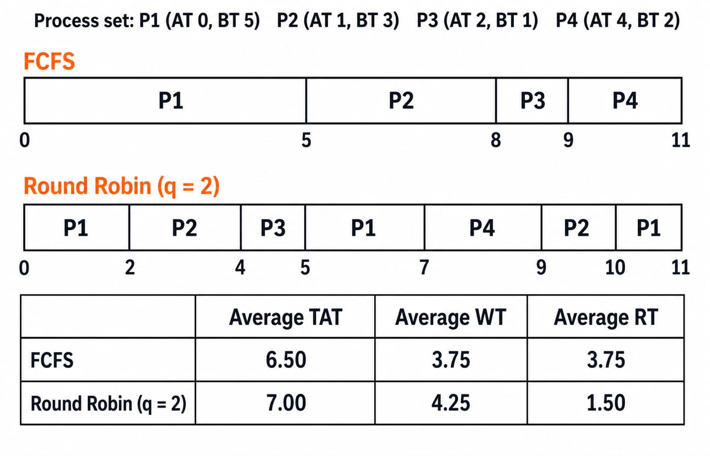
Assume one CPU, no I/O, zero switching cost and Round Robin q = 2. At a quantum boundary, enqueue new arrivals before the expired process.
FCFS calculation
FCFS runs P1 0-5 | P2 5-8 | P3 8-9 | P4 9-11.
Process | CT | TAT | WT | RT |
|---|---|---|---|---|
P1 | 5 | 5 | 0 | 0 |
P2 | 8 | 7 | 4 | 4 |
P3 | 9 | 7 | 6 | 6 |
P4 | 11 | 7 | 5 | 5 |
Average TAT = (5 + 7 + 7 + 7) / 4 = 26 / 4 = 6.50. Average WT = (0 + 4 + 6 + 5) / 4 = 15 / 4 = 3.75. Average RT = (0 + 4 + 6 + 5) / 4 = 15 / 4 = 3.75.
Without idle time or overhead, utilisation is 11 / 11 × 100 = 100% and throughput is 4 / 11, about 0.364 processes per time unit.
Round Robin calculation
The boundary rule gives P1 0-2 | P2 2-4 | P3 4-5 | P1 5-7 | P4 7-9 | P2 9-10 | P1 10-11.
Process | CT | TAT | WT | RT |
|---|---|---|---|---|
P1 | 11 | 11 | 6 | 0 |
P2 | 10 | 9 | 6 | 1 |
P3 | 5 | 3 | 2 | 2 |
P4 | 9 | 5 | 3 | 3 |
Average TAT = (11 + 9 + 3 + 5) / 4 = 28 / 4 = 7.00. Average WT = (6 + 6 + 2 + 3) / 4 = 17 / 4 = 4.25. Average RT = (0 + 1 + 2 + 3) / 4 = 6 / 4 = 1.50.
With zero overhead, utilisation stays 100% and throughput stays 4 / 11, about 0.364. Here FCFS lowers waiting and turnaround averages, while Round Robin lowers first response. Neither always wins.
CPU utilisation and throughput: an overhead check
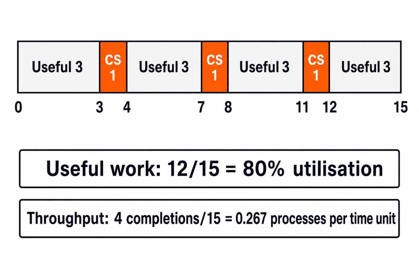
Four processes perform 12 useful units, with three 1-unit switches and no idle gap. Elapsed time is 12 + 3 = 15.
Utilisation is 12 / 15 × 100 = 80% and throughput is 4 / 15, about 0.267 processes per time unit. With zero switch cost, they become 100% and 4 / 12, about 0.333 processes per time unit.
A shorter quantum may improve response but hurt utilisation and throughput. Include switching, dispatch latency and idle gaps only when stated non-zero.
CPU scheduling calculation traps that change the answer
CT is an absolute finishing time, while TAT is CT - AT.
RT uses only the first start. WT counts every stay in the ready queue.
Track arrivals during execution. Never select a process before arrival.
State the tie rule for equal arrivals, equal priorities and quantum-boundary events.
A safe average does not rule out starvation; 100% utilisation does not imply good response.
For P2 under Round Robin, TAT = 10 - 1 = 9, WT = 9 - 3 = 6, but RT = 2 - 1 = 1. It then waited after preemption.
Throughput matches only because both finish 11 useful units at time 11 without overhead. Switching or idle time can change it.
CPU scheduling exam patterns and a practice sequence
Common forms include definitions, Gantt-chart numericals, objective-based comparisons, and variants with priorities, I/O, quantum or switching cost. KnowledgeGate has about 50 questions currently available for practice in CPU Scheduling, Basics & Criteria.
Use four passes: write AT and BT; trace queue and Gantt chart; calculate CT, then derived metrics; check units, ties, idle gaps and overhead. Change one assumption and recalculate.
For a broad four-policy comparison, use CPU scheduling algorithms: FCFS, SJF, Round Robin and priority explained. CPU Scheduling in Operating Systems: Algorithms, Gantt Charts and Worked Examples continues into SRTF, multilevel queues and MLFQ. Round Robin Scheduling Explained: Gantt Charts, Waiting Time and GATE Traps traces every queue update and switch-cost variant, while the paired chart above isolates its response-time trade-off against FCFS.
CPU scheduling basics: the short version and next step
Build the timeline, calculate CT, then derive TAT, WT and RT. Judge a named criterion and include only stated overhead. Here Round Robin cuts average response from 3.75 to 1.50, while FCFS keeps lower waiting and turnaround averages.
For a complete subject sequence, continue with GATE Guidance by Sanchit Sir. Then redraw both charts, calculate every row, and compare response with waiting.
Go deeper with the full courseOperating System
Keep learning

CPU Scheduling Basics and Criteria MCQs: 12 Solved Questions with Explanations
Attempt 12 CPU scheduling MCQs, then check concise explanations, an FCFS metric map, and three calculations built carefully from units.
Updated 30 Oct 20267 min readOperating System MCQs
Neural Network Architectures Interview Questions: Worked Answers and Trade-offs
Build speakable answers about MLPs, CNNs, recurrent models, Transformers, residual blocks and encoder-decoder systems through exact worked examples.
Updated 17 Nov 20266 min readInterview Corner
C# vs C++: Managed .NET, Native Control, and the Trade-offs That Matter
Compare one component in C# and C++, then use its lifetime, generic, build, and interop behaviour to choose the right model for your software.
Updated 23 Sep 20266 min readProgramming Languages Survey

Rust vs C++: Compare Safety, Control and Developer Trade-offs
Compare how Rust and modern C++ express ownership, catch lifetime mistakes, measure iterator code and define safe foreign-function boundaries.
Updated 19 Sep 20266 min readProgramming Languages Survey