

Neural Network Architectures Interview Questions: Worked Answers and Trade-offs
Build speakable answers about MLPs, CNNs, recurrent models, Transformers, residual blocks and encoder-decoder systems through exact worked examples.
KnowledgeGate Team
Exam prep & CS education
Updated 17 Nov 20266 min read
Candidates often memorise that CNNs suit images, RNNs suit sequences and Transformers use attention, but that list breaks down under follow-up questions. Architecture answers become stronger when you tie each model to its information flow, compute and constraints. A useful interview response connects the input structure to the model's inductive bias, traces one calculation and names a trade-off. These prompts apply across employers; they are not a company-specific question list.
What is a neural network architecture? Give the 30-second interview answer
A neural network architecture is the model's organised computation graph: its layers, information flow, parameter sharing and built-in structural bias. It differs from training configuration. An optimiser and learning rate govern parameter updates; dense connectivity, convolution, recurrence, attention, residual paths and encoder-decoder structure define the network.
A strong short answer is: an MLP connects features through dense layers; a CNN shares local filters across a grid; an RNN carries state through an ordered sequence; and a Transformer lets tokens exchange information through attention. Residual and encoder-decoder designs alter information flow through depth or from input to output. The right choice depends on the data, task, latency, memory and training data. For neuron fundamentals, forward passes and backpropagation, see the earlier Artificial Neural Networks Interview Questions and Answers; this post concentrates on architecture choice and structural trade-offs.
How do you choose an architecture from the input and task?
Reason from input geometry to useful invariance or dependency, constraints, candidate architecture and validation.
Problem | Input shape | Reasonable starting architecture | Structural reason | Caveat |
|---|---|---|---|---|
Binary classification | 24 standardised tabular features | MLP | Dense interaction across features | Tree models are also a baseline |
Ten-class images |
| CNN | Local filters and spatial weight sharing | Augmentation and data volume still matter |
Sensor windows |
| 1D CNN, GRU or Transformer | Local patterns, state or content-dependent interactions | Sequence length and resource budget decide the trade-off |
Text sequences | Up to | Transformer with positional information | Content-dependent token interactions | Data, latency and memory still constrain the choice |
These are starting points, not guaranteed winners. The Artificial Intelligence (AI) course is an optional structured learning route.
CNN versus dense layer: calculate the parameter difference exactly
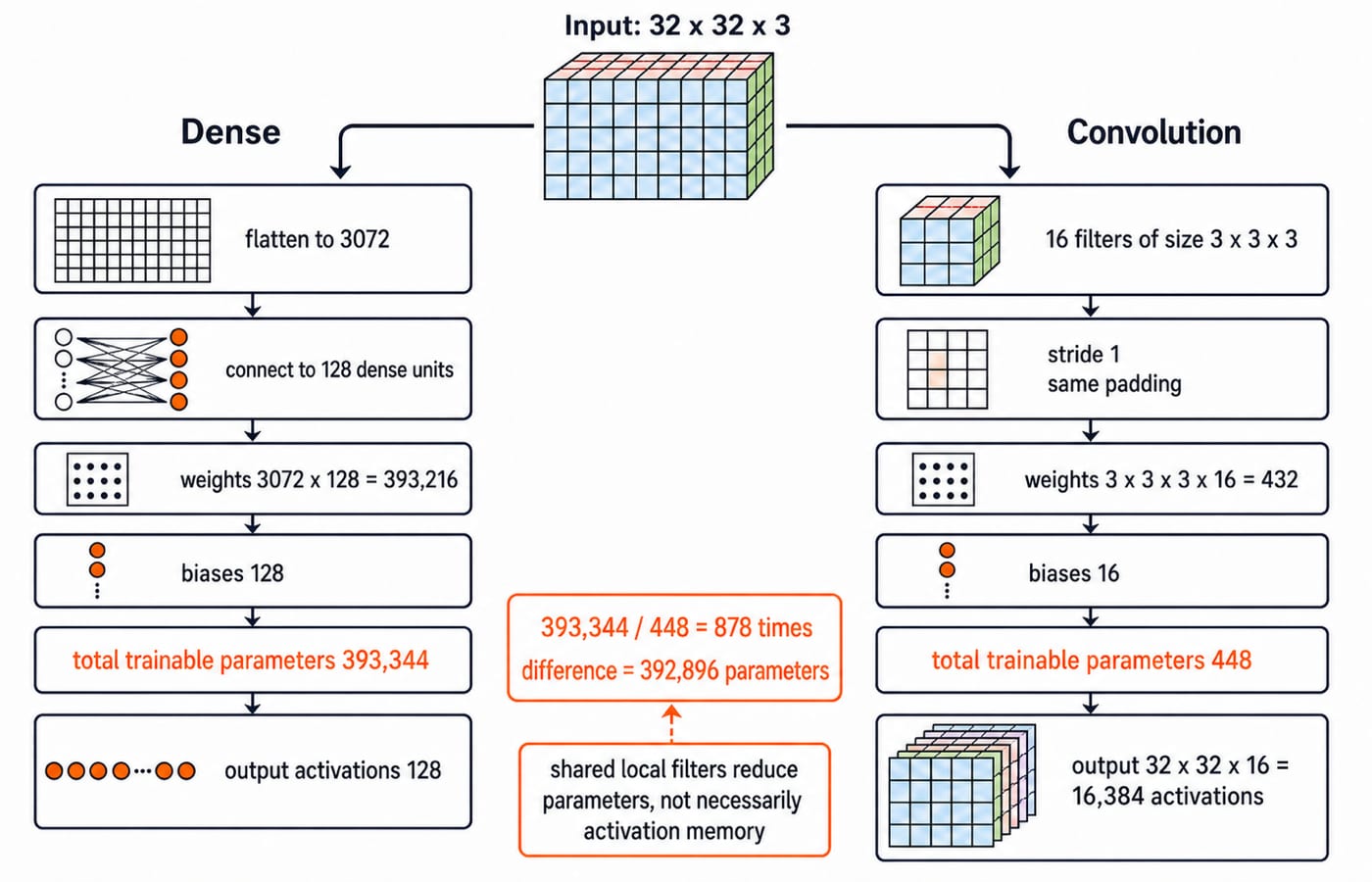
Prompt: an input image has shape 32 x 32 x 3. Option A flattens it to 3,072 values and connects it to 128 dense units, with one bias per unit.
The weight count is 3,072 x 128 = 393,216. Adding 128 biases gives 393,216 + 128 = 393,344 trainable parameters and 128 output activations.
Option B applies 16 filters of size 3 x 3, with stride 1, same padding and one bias per filter. Its count is 3 x 3 x 3 x 16 + 16 = 432 + 16 = 448 parameters. Its output is 32 x 32 x 16, which contains 16,384 activations. Therefore, the dense layer has 393,344 / 448 = 878 times as many parameters, a difference of 393,344 - 448 = 392,896.
The CNN reuses each filter's 3 x 3 x 3 weights at every spatial position. The dense layer learns a separate connection from every flattened pixel-channel value to every unit. Fewer parameters does not mean fewer stored activations here, since 16,384 > 128, and it alone proves neither faster execution nor better accuracy.
RNN, LSTM, GRU or Transformer: what changes for a sequence?
An exact scalar trace makes recurrence visible. Let h_0 = 0, (x_1, x_2, x_3) = (1, 2, -1) and h_t = tanh(0.5x_t + 0.8h_(t-1)).
z_1 = 0.5(1) + 0.8(0) = 0.500000, soh_1 = tanh(0.500000) = 0.462117.z_2 = 0.5(2) + 0.8(0.462117) = 1.369694, soh_2 = tanh(1.369694) = 0.878622.z_3 = 0.5(-1) + 0.8(0.878622) = 0.202898, soh_3 = tanh(0.202898) = 0.200159.
The same parameters 0.5 and 0.8 are reused at every step, while the hidden state represents the ordered prefix. A basic RNN can struggle with long gradient paths. LSTM and GRU add gates that control writing, keeping and exposing state. A Transformer replaces the single recurrent chain with attention between token representations and needs positional information for order.
Ask about sequence length, streaming or full-context inference, training data, latency and memory. Parallel training does not mean constant compute or memory, and an autoregressive decoder still generates successive output tokens during inference.
How does self-attention mix information? Work a two-token answer
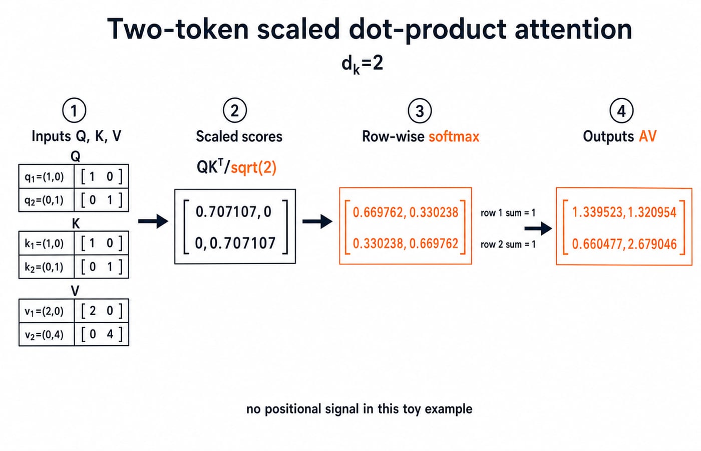
Consider one attention head with d_k = 2: q_1 = (1,0), q_2 = (0,1), k_1 = (1,0), k_2 = (0,1), v_1 = (2,0) and v_2 = (0,4). Each score is q_i dot k_j / sqrt(2).
For token 1, the scores are (0.707107, 0). Row-wise softmax gives (0.669762, 0.330238), so its output is:
0.669762v_1 + 0.330238v_2 = (1.339523, 1.320954).
For token 2, the scores are (0, 0.707107) and the weights are (0.330238, 0.669762). Its output is:
0.330238v_1 + 0.669762v_2 = (0.660477, 2.679046).
Each result is a content-dependent weighted sum, not a one-token lookup. Dividing by sqrt(d_k) controls dot-product scale as key dimension grows. Softmax makes the displayed weights positive and each row sum to 1.
This toy uses one head, two tokens and hand-chosen Q, K and V; it is neither a trained model nor a production-cost example. With no positional signal, swapping token order merely swaps the corresponding rows. Real sequence models add positional information or another order-aware mechanism.
What do residual and encoder-decoder connections solve?
A residual block learns F(x) and commonly uses y = ReLU(F(x) + x). If x and F(x) are both 56 x 56 x 64, element-wise addition works. If downsampling makes F(x) equal to 28 x 28 x 128, raw x cannot be added. A no-bias 1 x 1, stride-2 projection maps 64 channels to 128, contains 1 x 1 x 64 x 128 = 8,192 weights and produces 28 x 28 x 128.
An encoder builds an input representation; a decoder produces a target structure conditioned on it. Translation and image segmentation use this broad idea with different connection patterns. Residual addition requires matching shapes. Concatenation instead increases the channel or feature dimension, and not every skip connection is a residual addition.
Architecture follow-ups and traps that expose shallow answers
Is deeper always better? No. Data, optimisation, regularisation, compute and latency can make extra depth unhelpful.
Are CNNs only for images? No. Convolution models local structure in 1D signals and other grids.
Does attention know order automatically? Not in the position-free toy operation above.
Are LSTM and GRU optimisers? No. They are gated recurrent architectures.
Does parameter count equal activation memory? No. Our CNN has
448parameters but16,384output activations.
Use two rehearsal depths. Depth A gives a 30-second definition and one selection reason. Depth B adds shapes, an exact calculation, one failure mode and one constraint. An interviewer at a service-based or product-based employer may ask either depth; there is no fixed company taxonomy here.
After tracing the architectures, use the ANN solved MCQs as a quick concept check.
Neural network architectures: the 45-second answer and next step
Choose by the structure that should be reused or connected. Dense layers mix features, convolutions share local filters, recurrent models carry ordered state, attention mixes token information by learned relevance, residual paths help information cross depth, and encoder-decoder systems map an input representation to structured output. Data shape, dependency length, latency, memory and validation evidence decide.
Reproduce 393,344 versus 448 and one attention row without notes. The Interview & Resume Preparation Course is an optional spoken-answer route; the Placement Preparation & Coding track is the broader catalog.
Keep learning
Neural Network Architectures: Layers, Forward Passes and Worked Examples
Learn to read dense, convolutional and recurrent network diagrams as calculations. Count parameters, follow an exact 2-2-1 forward pass, and see what sharing changes.
Updated 4 Nov 20266 min readML & Data Science

DBMS Scenario Questions: Schema Design, Indexing and Concurrency Trade-offs
Use one course-enrolment case to practise the reasoning behind normalisation, composite indexes and safe concurrent seat allocation.
Updated 13 Sep 20266 min readInterview Corner

CPU Scheduling Basics and Criteria: Metrics, Trade-offs and Worked Examples
Learn how the ready queue, scheduler and dispatcher shape a CPU timeline, then calculate CT, TAT, WT and RT for FCFS and Round Robin on the same process set.
Updated 29 Oct 20265 min readOperating Systems

C# vs C++: Managed .NET, Native Control, and the Trade-offs That Matter
Compare one component in C# and C++, then use its lifetime, generic, build, and interop behaviour to choose the right model for your software.
Updated 23 Sep 20266 min readProgramming Languages Survey