

Transportation Problem Optimality Test with the MODI Method: Step-by-Step Worked Example
Follow one balanced transportation problem from a north-west corner solution costing 80 through one MODI improvement loop to a unique optimum costing 50.
KnowledgeGate Team
Exam prep & CS education
Updated 19 Nov 20265 min read

Once you have an initial basic feasible solution, the transportation table may look complete. But feasible does not automatically mean cheapest. MODI often feels confusing because potentials, opportunity-cost signs, and the closed loop are taught as separate procedures. A balanced minimisation example runs from its initial cost through one improvement loop to a proved optimum. Track every potential, allocation change, and cost calculation. The MODI procedure is reproducible when each calculation follows from the current basis.
What the MODI optimality test actually checks
A feasible transportation plan satisfies every source supply and every destination demand. The MODI optimality test asks a different question: can units move around a closed loop to reduce cost while all those totals remain unchanged?
For an (m x n) non-degenerate solution, the basis must contain exactly (m+n-1) basic cells. At each basic cell, write
u_i + v_j = c_ij.
Choose one potential, usually (u_1=0), and solve the connected equations for the others. This is the same disciplined equation-solving habit used in Linear Algebra for GATE CS.
Use one sign convention throughout: for every unoccupied cell,
Delta_ij = c_ij - (u_i + v_j).
For minimisation, the current plan is optimal when every Delta_ij >= 0. A negative value identifies an improving cell. Some books define the difference in the reverse order, in which case their stopping inequality must reverse too.
Set up a balanced table and its initial basis
Consider this transportation cost table:
Source | D1 | D2 | D3 | Supply |
|---|---|---|---|---|
S1 | 2 | 7 | 4 | 5 |
S2 | 3 | 3 | 1 | 8 |
S3 | 5 | 4 | 7 | 7 |
Demand | 6 | 8 | 6 | 20 |
Total supply is 5+8+7=20, and total demand is 6+8+6=20, so the problem is balanced.
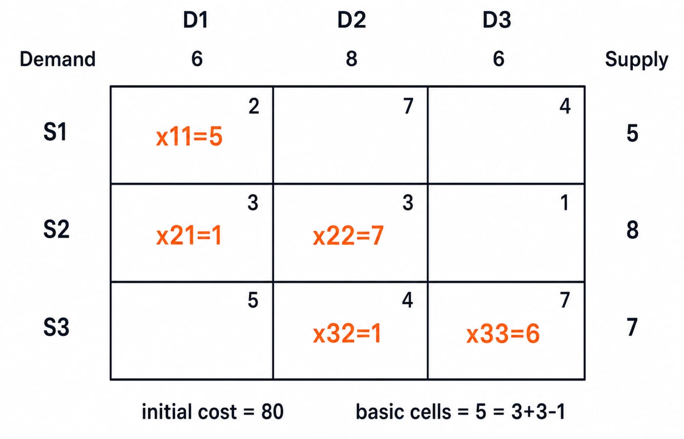
The north-west corner rule gives x_11=5, x_21=1, x_22=7, x_32=1, and x_33=6. Every other shipment is zero and non-basic at this stage. The row totals are 5, 1+7=8, and 1+6=7. The column totals are 5+1=6, 7+1=8, and 6. All supplies and demands are satisfied.
There are five positive basic cells, exactly 3+3-1=5, so this basis is non-degenerate. Its initial cost is
5(2)+1(3)+7(3)+1(4)+6(7)=10+3+21+4+42=80.
The north-west corner rule uses only the positions of supply and demand, not the costs. Therefore, 80 is a feasible starting value, not proof of a minimum.
Compute potentials and find the entering cell
Set u_1=0. Use only basic cells in u_i + v_j = c_ij, moving through the connected basis:
Basic cell | Equation | Derived potential |
|---|---|---|
x_11 | 0+v_1=2 | v_1=2 |
x_21 | u_2+2=3 | u_2=1 |
x_22 | 1+v_2=3 | v_2=2 |
x_32 | u_3+2=4 | u_3=2 |
x_33 | 2+v_3=7 | v_3=5 |
Each result comes from a basic-cell equality with one known potential. The connected five-cell basis lets values propagate without borrowing an equation from an unoccupied cell.
Thus u=(0,1,2) and v=(2,2,5). Now calculate every unoccupied-cell opportunity cost:
Delta_12=7-(0+2)=5,
Delta_13=4-(0+5)=-1,
Delta_23=1-(1+5)=-5,
Delta_31=5-(2+2)=1.
Positive values at x_12 and x_31 offer no reduction. Negative values at x_13 and x_23 mark possible improvements.
The plan is not optimal because two values are negative. Choose x_23 as the entering cell because -5 is the most negative opportunity cost. It shows the cost change per unit moved through a valid loop. It is not, by itself, the final saving because the loop determines how many units can move.
Draw the closed loop, choose theta, and update allocations
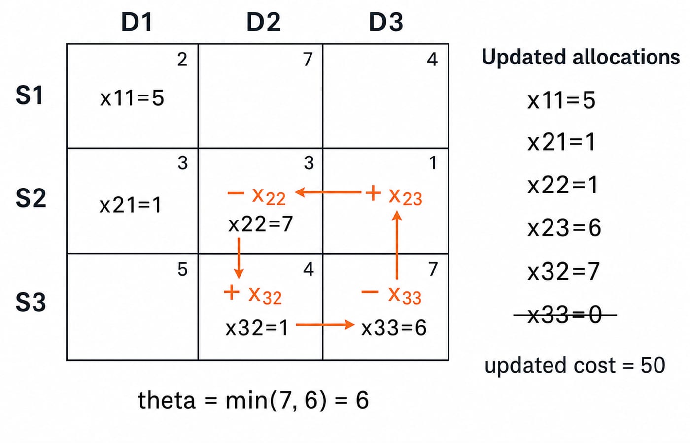
Starting at the entering cell, trace this rectangular loop:
x_23(+) -> x_22(-) -> x_32(+) -> x_33(-) -> x_23.
Every turn occurs at a basic cell, and signs alternate after the plus sign at the entering cell. The minus positions control the allowable shift:
theta = min(x_22 = 7, x_33 = 6) = 6.
Taking theta from the minus cells prevents negative shipments. Any shift above 6 would make x_33 negative. Each affected row and column has one plus and one minus corner, so its supply or demand total stays fixed. This preserves balance exactly.
Add 6 at plus positions and subtract 6 at minus positions:
x_23=0+6=6
x_22=7-6=1
x_32=1+6=7
x_33=6-6=0
Drop x_33 from the basis and admit x_23. The unchanged allocations are x_11=5 and x_21=1. The updated basis still has five positive allocations. Supplies now total 5, 1+1+6=8, and 7. Demands total 5+1=6, 1+7=8, and 6. Feasibility is preserved.
The new cost is
5(2)+1(3)+1(3)+6(1)+7(4)=10+3+3+6+28=50.
The cost change is theta x Delta_23=6(-5)=-30, so the saving is 30, matching the fall from 80 to 50.
Run MODI again and prove that 50 is optimal
The new basis is x_11, x_21, x_22, x_23, x_32. Again set u_1=0. The basic-cell equations give v_1=2 from x_11, u_2=1 from x_21, v_2=2 from x_22, v_3=0 from x_23, and u_3=2 from x_32. Notice that v_3 changes because x_23, not x_33, now connects destination D3 to the basis.
For the four unoccupied cells:
Delta_12=7-(0+2)=5,
Delta_13=4-(0+0)=4,
Delta_31=5-(2+2)=1,
Delta_33=7-(2+0)=5.
Every opportunity cost is positive. Even the smallest, Delta_31=1, would increase cost rather than reduce it if that route entered through its loop. No cost-reducing loop remains, so the minimum transportation cost is 50. All five basic allocations are positive, making the basis non-degenerate, and every non-basic opportunity cost is strictly positive. Therefore this example has a unique optimum. The evidence is complete. If an unoccupied cell instead had Delta=0, it would signal an alternate optimum.
MODI traps that change the answer
Error: Pair our Delta definition with a non-positive stopping rule. Consequence: The decision reverses. Correction: Stop at non-negative values.
Error: Use non-basic cells for potentials. Consequence: The equations misrepresent the basis. Correction: Use its m+n-1 basic cells.
Error: Choose theta from plus cells. Consequence: A minus allocation may become negative. Correction: Use minus positions, which gave theta=6.
Error: Draw a diagonal or open path. Consequence: Totals change. Correction: Close a right-angled loop through basics with alternating signs.
A plan with fewer than m+n-1 basics is degenerate. Place an infinitesimal epsilon in an independent zero-allocation cell to connect the potential equations, treating its shipment as zero in costs and totals. Balance unequal totals with a zero-cost dummy row or column. A zero Delta indicates an alternate optimum, not an error.
How exam-style questions test MODI
Common question shapes are:
Decide whether a supplied basic plan is optimal.
Identify the entering cell, closed loop, and theta.
Calculate the new minimum cost after one or more iterations.
Watch for a reversed opportunity-cost convention, a degenerate basis, or a zero reduced cost. For a timed self-check, hide this solution and recover u=(0,1,2), v=(2,2,5), entering cell x_23, the four-corner loop, and cost 50. Work under a short timer and mark the first step where your result differs. KnowledgeGate has a few live practice questions on transportation-problem optimality, so use them to test the method after you can reproduce these numbers unaided.
The short version and the next practice step
Use six actions: confirm balance; count m+n-1 basics; solve u_i + v_j = c_ij; compute every unoccupied Delta_ij; improve through the most negative cell and a valid loop; repeat until all values are non-negative. Keep that checklist beside you for the next hand calculation. Continue with Engineering Mathematics for GATE, use GATE Guidance by Sanchit Sir for broader preparation, or browse the GATE course category. For another numerical explainer, read Probability for GATE CS.
Go deeper with the full courseEngineering Mathematics for GATE Exam
Keep learning

Transportation Problem Formulation: Balanced and Unbalanced Cases with Worked Examples
Learn how to define variables and constraints, test balance, add the correct dummy destination or source, and verify complete feasible allocations in two linked examples.
Updated 18 Nov 20265 min readEngineering Mathematics

Graphical Method in Linear Programming: Feasible Region, Corner Points and Optimality with a Worked Example
Learn the two-variable graphical method in the right order, then solve and audit a complete maximisation model without trusting the sketch alone.
Updated 21 Oct 20265 min read73 viewsEngineering Mathematics

Assignment Problem and Hungarian Method: Formulation with a Complete Worked Example
Learn why greedy assignment fails, how matrix reductions preserve the optimum, and how the uncovered-value adjustment leads to a minimum cost of 140.
Updated 24 Sep 20266 min read62 viewsEngineering Mathematics
Linear Programming Problem Structure and Mathematical Model: A Step-by-Step Worked Example
Learn how to turn a word problem into an LP model, check feasibility, find every corner point, and identify the optimum in one consistent numerical example.
Updated 14 Nov 20265 min readEngineering Mathematics