Graphical Method in Linear Programming: Feasible Region, Corner Points and Optimality with a Worked Example
Learn the two-variable graphical method in the right order, then solve and audit a complete maximisation model without trusting the sketch alone.
KnowledgeGate Team
Exam prep & CS education
Updated 21 Oct 20265 min read
You can draw both boundary lines correctly and still shade the wrong half-planes. You can also miss the corner where two lines meet, or pick the point that looks farthest without ever testing the objective. In a graphical linear-programming solution, convert inequalities into a common region, identify corner points, evaluate objective values, and confirm the result with an objective line.
What the graphical method solves, and the vocabulary to keep separate
A two-variable linear programme has decision variables such as x and y, a linear objective such as Z=3x+5y, linear constraints, and usually non-negativity restrictions. Replacing an inequality by equality gives its boundary line. The inequality itself selects one half-plane bounded by that line.
Keep three ideas separate. The feasible region is the intersection of every allowed half-plane. A corner point, or extreme point, is a vertex of that region. An optimal solution is a feasible point giving the best objective value. A feasible point need not be a corner, and a corner need not be optimal.
Optimization in Discrete Mathematics is the broad survey: it compares continuous LP with integer, assignment, transportation and network models. This page stays with the two-variable graph itself: half-plane shading, exact vertices, objective-line movement and special geometric outcomes. For the surrounding exam syllabus, use the GATE CS exam-preparation category.
Turn each inequality into a boundary line and locate the feasible region
Use the same coefficient set as Duality in LP, where it constructs the dual and certifies objective value 21 algebraically. Here the coefficients are used to build and audit the graph:
Maximise Z=3x+5y, subject to x+2y<=8, 3x+2y<=12, x>=0, and y>=0.
Non-negativity first restricts the graph to the first quadrant. Replace each sloping inequality by equality and find its intercepts:
Boundary line | x-intercept | y-intercept |
|---|---|---|
|
|
|
|
|
|
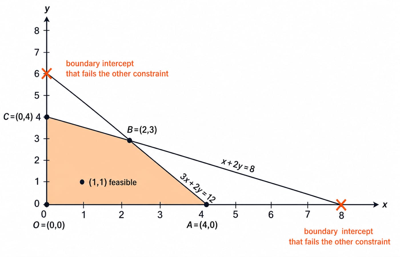
Draw the complete boundary lines, not only the intercept segments. Both constraints use <=, so test (0,0). It gives 0<=8 and 0<=12; therefore, shade the origin side of each line. Their overlap in the first quadrant is the feasible region.
Check (1,1): 1+2=3<=8 and 3+2=5<=12, so it is feasible. In contrast, (8,0) fails the second constraint because 3(8)+2(0)=24>12. The point (0,6) fails the first because 0+2(6)=12>8.
Find every corner point before evaluating the objective
Generate candidates from active-boundary pairs instead of guessing from the picture. The axes meet at (0,0). On y=0, the binding sloping constraint is 3x+2y=12, which gives (4,0). On x=0, the binding constraint is x+2y=8, which gives (0,4).
Now solve the two sloping boundaries together, without reading rounded coordinates from the graph:
Subtract
x+2y=8from3x+2y=12:2x=4, sox=2.Substitute into
x+2y=8:2+2y=8, so2y=6andy=3.Thus, the intersection is
(2,3). It satisfies both original inequalities at equality.
The ordered feasible-corner list is (0,0), (4,0), (2,3), (0,4). The intercepts (8,0) and (0,6) are rejected because each violates the other constraint. The point (1,1) is feasible but is not a vertex. For the algebraic distinction among basic solutions, BFS points and optimal solutions, see Basic Terminologies in Linear Programming; graphical corner enumeration uses only feasible boundary intersections.
Use this audit every time: generate boundary intersections, test each candidate against every original constraint, discard infeasible candidates, then remove feasible points that do not form vertices. A pairwise line intersection is not automatically a corner.
Evaluate corner points and confirm the unique optimum geometrically
Substitute every feasible corner into the objective:
Corner |
| Result |
|---|---|---|
|
| feasible corner |
|
| feasible corner |
|
| unique maximum |
|
| feasible corner |
Therefore, Zmax=21 at (2,3). The corner-point principle says that if a linear objective has a finite optimum over a non-empty polygonal feasible region, at least one optimum occurs at a corner. It does not say that every LP has a unique optimum.
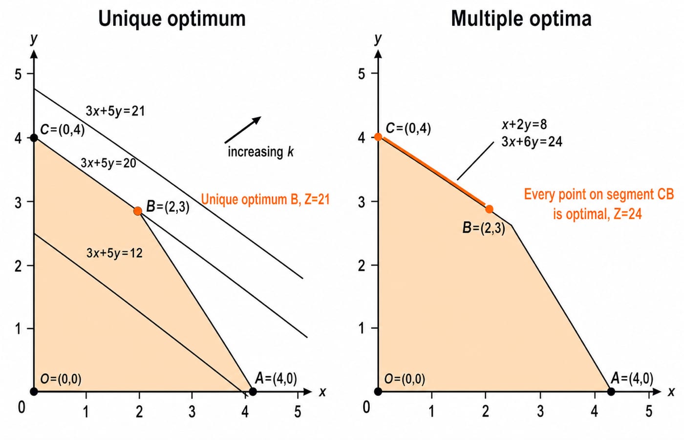
The objective lines 3x+5y=k all have slope -3/5. As k increases, slide the line in direction (3,5). Its last contact with this polygon is the single vertex (2,3) on 3x+5y=21. The adjacent edges have slopes -3/2 and -1/2, neither equal to -3/5, so the objective line cannot overlap either edge.
Alternate optima, infeasibility and unboundedness as geometric outcomes
Keep the constraints but change the objective to maximise Z'=3x+6y=3(x+2y). Both (0,4) and (2,3) give 24. Every point on the feasible segment joining them satisfies x+2y=8, so every such point also gives 24. There are infinitely many optimal solutions. Geometrically, the moving objective line is parallel to, and finally coincides with, a binding feasible edge.
For infeasibility, consider x+y<=2, x+y>=4, with x,y>=0. The same sum cannot be at most 2 and at least 4. The allowed half-planes never overlap, so there is no feasible region and no optimum.
For unboundedness, maximise Z=x+y subject to x-y>=0, x,y>=0. For every t>=0, (t,t) is feasible and gives Z=2t. Since t can increase without limit, there is no finite maximum. However, an unbounded feasible region does not make every objective unbounded. The objective must improve indefinitely along a feasible direction.
Graphical-method mistakes and the repair for each one
Mistake | What goes wrong | Repair |
|---|---|---|
Shading by the equality line alone | A line has two sides | Test |
Ignoring | Extra quadrants create false corners | Impose the first quadrant |
Keeping | Each satisfies only its own boundary | Retest against every constraint |
Reading | Rounding can change objective comparisons | Solve line intersections algebraically |
Checking only intercepts | The decisive corner | Include every active-boundary intersection |
Choosing the visually farthest point | Distance from the origin is not the objective | Evaluate |
One wording trap remains. In a minimisation problem, “optimal” means the smallest feasible objective value. It does not automatically mean the top-right or bottom-left point on the picture.
How questions test the graphical method
Representative tasks ask you to identify a feasible region from several plots, calculate a missing corner, choose a maximum or minimum from a corner table, detect alternate optima from parallel slopes, classify a model as infeasible or unbounded, or test a proposed point for feasibility. Each one reduces to the same audit, so practise the audit rather than one memorised picture.
Run this 60-second audit on the worked model:
boundaries -> correct half-planes -> common region -> candidates -> feasibility recheck -> corner table -> objective-line confirmation
Your checkpoints must be O(0,0), A(4,0), B(2,3), C(0,4), followed by objective values 0,12,21,20. If one number differs, return to the line intersection or substitution before trusting the sketch.
Graphical method short version and the next useful step
Draw equality boundaries, choose each allowed half-plane, intersect them with non-negativity, solve and verify every corner, evaluate the objective, then move the objective line to recognise one best vertex or a full optimal edge. Here the feasible corners are (0,0), (4,0), (2,3), (0,4), and the unique maximum is Z=21 at (2,3).
Now redraw the polygon and reconstruct the four-row objective table without looking. Engineering Mathematics for GATE Exam offers a broader mathematics foundation for the surrounding syllabus.
Keep learning

Duality in LP: Construct the Dual, Solve a Worked Example, and Apply Key Properties
Learn a reliable matrix-first method to form an LP dual, solve both programs to value 21, and use duality properties to check optimality and avoid sign errors.
Updated 17 Oct 20266 min readEngineering Mathematics

Commutative Property and Abelian Groups: Tests, Worked Examples and Exam Traps
Learn how to separate commutativity from the other group axioms, test custom operations step by step, and avoid the usual classification traps.
Updated 13 Oct 20266 min readEngineering Mathematics

Closure, Semigroup and Monoid: Worked Algebraic Structure Examples
Learn a reliable order for testing closure, associativity and identity. Worked tables and counterexamples show exactly when a structure becomes a semigroup or monoid.
Updated 9 Oct 20266 min readEngineering Mathematics
Classification of Finite and Infinite Groups: Orders, Cyclicity and Worked Examples
Learn how group axioms, group order, element order and generators classify finite and infinite groups through complete, checkable examples.
Updated 4 Oct 20266 min readEngineering Mathematics