

Transportation Problem Formulation: Balanced and Unbalanced Cases with Worked Examples
Learn how to define variables and constraints, test balance, add the correct dummy destination or source, and verify complete feasible allocations in two linked examples.
KnowledgeGate Team
Exam prep & CS education
Updated 18 Nov 20265 min read
A transportation table looks like arithmetic, but the examinable work starts before allocation. You must define variables and constraints, compare total supply with total demand, and add the correct dummy row or column when they differ. Changing Z's demand from 15 to 12 turns the balanced table into a three-unit excess-supply case, a standard GATE CS exam preparation task.
What a transportation problem is, and what balanced means
A transportation problem sends units from supply sources to demand destinations. Let c_ij be the unit cost from source i to destination j, s_i the available supply, d_j the required demand, and non-negative x_ij the quantity shipped. The objective is to meet the requirements at minimum total cost, subject to the supply and demand assumptions: min Z = sum(c_ij x_ij).
Before using any solution method, calculate:
Total supply:
sum(s_i)Total demand:
sum(d_j)
Equal totals mean balanced; unequal totals mean unbalanced. Compare grand totals, not one row with one column. For wider optimisation context, see Engineering Mathematics.
Formulate the balanced transportation table
Each inner entry below is a unit transportation cost.
Source / destination | X | Y | Z | Supply |
|---|---|---|---|---|
A | 8 | 6 | 10 | 20 |
B | 9 | 7 | 4 | 30 |
Demand | 10 | 25 | 15 | 50 |
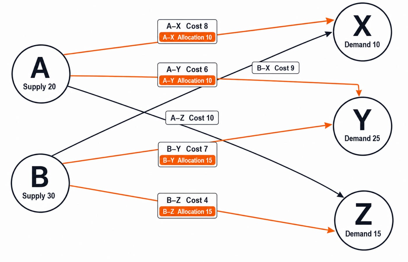
Total supply is 20 + 30 = 50. Total demand is 10 + 25 + 15 = 50. The problem is balanced.
Define x_AX, x_AY, x_AZ, x_BX, x_BY, and x_BZ; x_AY, for example, is the quantity from A to Y. The objective is:
min Z = 8x_AX + 6x_AY + 10x_AZ + 9x_BX + 7x_BY + 4x_BZ
The two source constraints are:
x_AX + x_AY + x_AZ = 20
x_BX + x_BY + x_BZ = 30
The three destination constraints are:
x_AX + x_BX = 10
x_AY + x_BY = 25
x_AZ + x_BZ = 15
Also, x_AX, x_AY, x_AZ, x_BX, x_BY, x_BZ >= 0. Divisible units need no integer restriction; indivisible shipments are a different modelling choice.
Check a complete allocation and calculate its cost
Send 10 units from A to X. X is satisfied, and A has 10 units left.
Send A's remaining 10 units to Y. Y still requires 15 units.
Send 15 units from B to Y. Y is now satisfied.
Send B's remaining 15 units to Z. Set the unused routes
x_AZandx_BXto zero.
Source checks:
A ships
10 + 10 + 0 = 20.B ships
0 + 15 + 15 = 30.
Destination checks:
X receives
10.Y receives
10 + 15 = 25.Z receives
15.
Z = (10 x 8) + (10 x 6) + (15 x 7) + (15 x 4)
Z = 80 + 60 + 105 + 60 = 305
Thus, 305 is the cost of this feasible plan. Feasibility does not prove optimality; initial-solution and optimality methods are separate next stages.
Convert an unbalanced table with a dummy source or destination
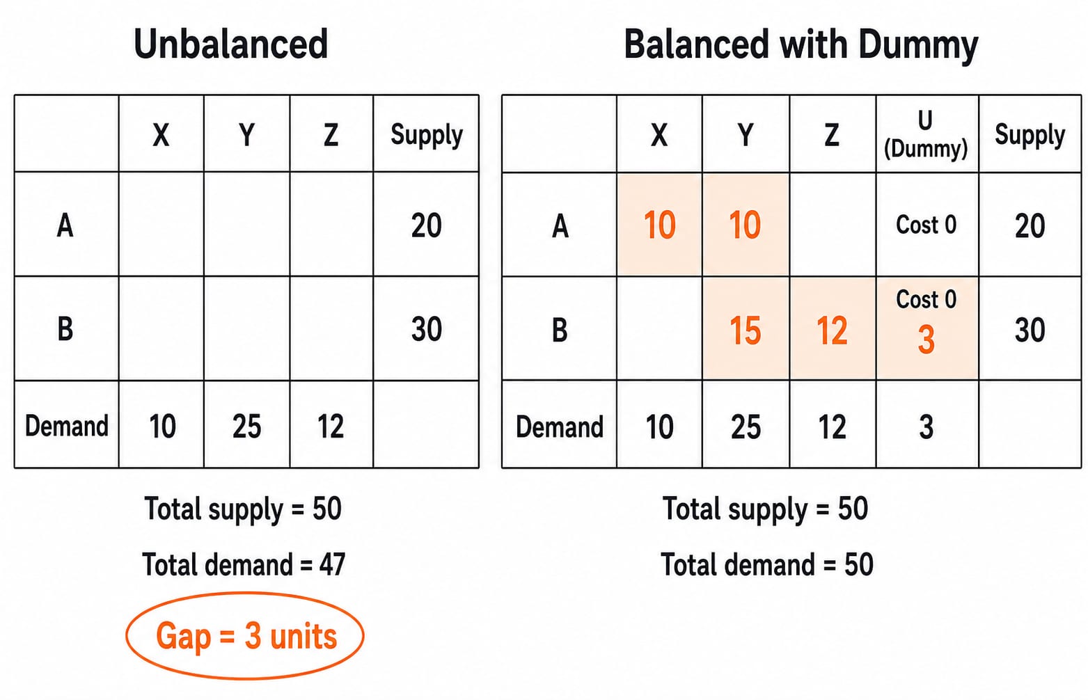
If supply is 50 and demand is 47, excess supply is
50 - 47 = 3. Add a dummy destination with demand 3.If supply is 40 and demand is 45, excess demand is
45 - 40 = 5. Add a dummy source with supply 5.
Dummy-destination allocation represents unused supply. Dummy-source allocation represents unmet demand in the table, not a physical shipment.
Use zero dummy costs only when no storage, wastage, shortage, or penalty cost is given. Otherwise use the stated penalty. A dummy is an accounting device that balances the model; it does not alter real capacity or demand.
Work the excess-supply variant with the same values
Change only Z's demand from 15 to 12. Supply remains 50, while demand becomes:
10 + 25 + 12 = 47
Add dummy destination U with demand 50 - 47 = 3 and costs A-U = 0, B-U = 0. The balanced 2 by 4 table has 8 decision variables.
x_AX = 10, x_AY = 10, x_BY = 15, x_BZ = 12, x_BU = 3
The remaining variables are x_AZ = 0, x_AU = 0, and x_BX = 0.
A ships 10 + 10 + 0 + 0 = 20; B ships 0 + 15 + 12 + 3 = 30. X, Y, Z, and U receive 10, 10 + 15 = 25, 12, and 3. Every total is satisfied.
The cost is:
Z = (10 x 8) + (10 x 6) + (15 x 7) + (12 x 4) + (3 x 0)
Z = 80 + 60 + 105 + 48 + 0 = 293
The 3 units assigned to U are unused supply, not customer delivery. The feasible plan costs 293; optimality is not implied.
Common formulation and balancing traps
Trap | Consequence | Correction |
|---|---|---|
Reversing supply and demand equations | Row and column meanings are lost | Write one equation per source row and one per destination column |
Comparing individual entries | A balanced table may be called unbalanced | Compare grand total supply with grand total demand |
Adding a dummy source for excess supply | The imbalance grows in the wrong direction | Add a dummy destination, which is a new column |
Treating dummy allocation as delivery | The plan receives a false physical meaning | Interpret it as unused supply or table-level unmet demand |
Assuming every dummy cost is zero | A stated shortage or storage cost disappears | Use the penalty supplied in the question |
Check that the objective minimises the given unit costs, variables are non-negative, and totals match after adding the dummy.
A balanced m x n table has m + n equality constraints, but one is redundant because the totals are equal. A non-degenerate basic feasible solution has m + n - 1 basic allocations. Here, 2 by 3 gives 2 + 3 - 1 = 4; after adding U, 2 by 4 gives 2 + 4 - 1 = 5. Fewer occupied basic cells mean degeneracy, not imbalance.
How exam-style questions test transportation formulation
Typical tasks ask you to identify balance, calculate and place a dummy, complete an objective or constraint, interpret dummy allocation, or separate feasibility from optimality.
Use this 30-second check sequence:
Add the grand supply and demand totals.
Find the dummy amount and its direction, if needed.
Check the table dimensions and variable count.
Write every source equation.
Write every destination equation.
Add non-negativity conditions.
Substitute allocations into the cost expression and recheck the arithmetic.
KnowledgeGate currently has about 4 live practice questions on this exact subtopic. The Discrete Mathematics MCQs guide supports broader practice, while the GATE Test Series offers timed, mixed-topic practice.
The short version and the next step
Define variables and cost, then compare total supply with total demand. Leave a balanced table unchanged. For imbalance, add a dummy destination for excess supply or dummy source for excess demand. Verify every row, column, and cost.
In the first table, supply 50 equals demand 50. In the variant, 50 against 47 requires dummy destination U with demand 3. That comparison decides whether balancing is needed.
For more practice, the Engineering Mathematics for GATE course is one structured option. Use these formulation rules when revising.
Go deeper with the full courseEngineering Mathematics for GATE Exam
Keep learning

Transportation Problem Optimality Test with the MODI Method: Step-by-Step Worked Example
Follow one balanced transportation problem from a north-west corner solution costing 80 through one MODI improvement loop to a unique optimum costing 50.
Updated 19 Nov 20265 min readEngineering Mathematics
Assignment Problem and Hungarian Method: Formulation with a Complete Worked Example
Learn why greedy assignment fails, how matrix reductions preserve the optimum, and how the uncovered-value adjustment leads to a minimum cost of 140.
Updated 24 Sep 20266 min read62 viewsEngineering Mathematics
IISc Administrative Assistant Preparation: A Balanced 10-Week Study Plan for Working Candidates
A practical ten-week system for working candidates, with diagnostic tests, balanced weekly blocks, error-led revision, mixed sets and mock analysis.
Updated 30 Oct 20266 min readIISC Administrative Assistant
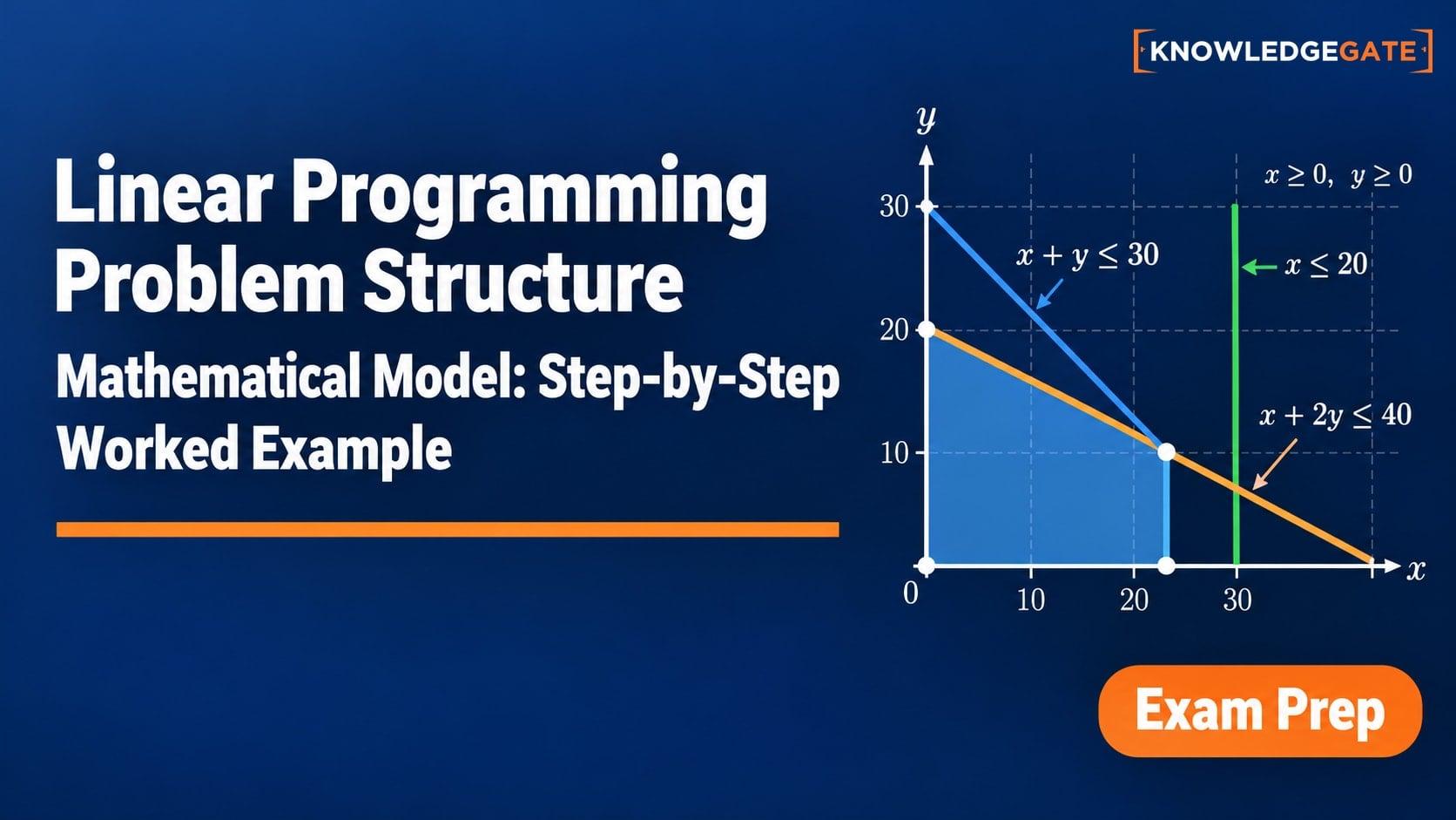
Linear Programming Problem Structure and Mathematical Model: A Step-by-Step Worked Example
Learn how to turn a word problem into an LP model, check feasibility, find every corner point, and identify the optimum in one consistent numerical example.
Updated 14 Nov 20265 min readEngineering Mathematics